Support our educational content for free when you purchase through links on our site. Learn more
Object Detection Algorithm Performance: 15 Metrics That Matter 🔍


Object detection algorithm performance is best judged by combining detection accuracy, localization quality, and real-world speed—not by trusting one mAP score. Compare models on representative data, check class-by-class errors, and benchmark them on the hardware you’ll actually deploy.
Why so many angles? CO-style evaluation averages precision across IoU thresholds from 0.50 to 0.95, revealing how a detector performs as box-localization requirements get stricter. A model can look impressive at a lenient threshold yet struggle to place tight boxes—or miss small, important objects entirely.
We’ve seen a “faster” detector lose its advantage once image decoding, preprocessing, and post-processing entered the timing test. That’s the catch: the algorithm is only one runner in a relay that ends with a real prediction on your device.
Key Takeaways
- Measure accuracy and efficiency together: report mAP, per-class precision and recall, latency, and throughput.
- Know what your metrics mean: IoU evaluates box overlap; AP summarizes a precision–recall curve; mAP averages AP across classes and, depending on the protocol, IoU thresholds.
- Benchmark fairly: keep the dataset, image size, hardware, thresholds, and evaluation method consistent.
- Inspect errors, not just scores: small objects, crowded scenes, poor labels, and domain shift can hide behind an aggregate result.
- Optimize for the application: choose thresholds and models based on the cost of false alarms, missed detections, latency, and compute.
- Test the full pipeline: preprocessing, inference, and post-processing all contribute to real-world performance.
Table of Contents
- ⚡️ Quick Tips and Facts
- 🧭 Object Detection Performance: Background and Evolution
- How object detection algorithms work
- Two-stage, one-stage, and transformer-based detectors
- 📏 15 Core Object Detection Performance Metrics
- 1. Intersection over Union (IoU)
- 2. True positives, false positives, and false negatives
- 3. Precision
- 4. Recall
- 5. F1 score
- 6. Precision–recall curve
- 7. Average precision (AP)
- 8. Mean average precision (mAP)
- 9. AP at a fixed IoU threshold
- 10. CO-style AP across IoU thresholds
- 11. AP by object size
- 12. Per-class performance
- 13. Inference latency
- 14. Throughput and frames per second
- 15. Model size and computational cost
- 🔍 How to Evaluate an Object Detection Model
- Prepare a representative dataset
- Check labels, bounding boxes, and class balance
- Choose evaluation splits and prevent data leakage
- Set confidence and IoU thresholds
- Build a reproducible evaluation pipeline
- 🧪 Benchmarking Detection Algorithms Fairly
- Compare models on the same data and hardware
- Measure end-to-end latency, not just model time
- Account for image size, batch size, and precision
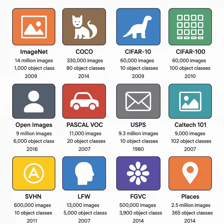
- Use established benchmarks: CO, Pascal VOC, and Open Images
- ⚖️ Accuracy Versus Speed: Choosing the Right Trade-Off
- Real-time object detection requirements
- Hardware considerations: GPU, CPU, edge, and mobile
- When a smaller model is the better choice
- 🛠️ What Affects Object Detection Algorithm Performance?
- Dataset quality, size, and domain shift
- Small objects, oclusion, and crowded scenes
- Architecture, backbone, and feature pyramids
- Input resolution, preprocessing, and augmentation
- Training settings, loss functions, and convergence
- Confidence calibration and non-maximum suppression
- 🚀 Practical Ways to Improve Detection Performance
- Improve data collection and annotation
- Tune thresholds and post-processing
- Optimize inference with quantization and acceleration
- Profile bottlenecks before changing the model
- 📊 Reading Results: Error Analysis and Diagnostics
- Confusion matrices and per-class errors
- Inspect false detections and missed objects
- Analyze performance across size, lighting, and conditions
- Spot overfitting and benchmark-to-production gaps
- 🤖 Comparing Popular Object Detection Algorithms
- Faster R-CNN and other two-stage detectors
- YOLO and other one-stage detectors
- SSD, RetinaNet, and efficient detectors
- DETR and transformer-based object detection
- 🏭 Production Deployment and Ongoing Monitoring
- Edge, cloud, and embedded deployment
- Monitor latency, accuracy, and data drift
- Set task-specific acceptance criteria
- ✅ Object Detection Performance Checklist
- 🏁 Conclusion
- 🔗 Recommended Links
- ❓ FAQ
- 📚 Reference Links
⚡️ Quick Tips and Facts
Object detection performance is not a single score. It’s the combination of what a model finds, how accurately it draws boxes, how often it makes mistakes, and how quickly it runs.
For a useful companion to this guide, start with our computer vision benchmarks overview. It helps put detector scores in context: a benchmark result is only meaningful when the dataset, evaluation rules, and hardware are clear.
| Quick fact | Why it matters |
|---|---|
| mAP summarizes detection quality across classes and confidence thresholds. | Useful for broad comparisons, but it can hide poor results on a critical class. |
| IoU measures the overlap between a predicted box and the annotated box. | A detection can identify the right object yet fail a strict localization threshold. |
| Precision and recall describe different error trade-offs. | Prioritize precision when false alarms are costly; prioritize recall when missed objects are dangerous. |
| Latency and throughput are different. | Latency is time per prediction; throughput is how many images or frames a system processes over time. |
| Input resolution affects accuracy and speed. | Larger images may preserve small objects but require more computation. |
| A benchmark score is not a deployment guarantee. | Camera angle, lighting, weather, hardware, and data drift can change real-world results. |
| Use the test set once for final evaluation. | Repeatedly tuning against test results turns the test set into an unofficial validation set. |
| Compare models under the same conditions. | Different image sizes, confidence thresholds, hardware, or post-processing settings can make a comparison unfair. |
A practical starting point: report CO-style mAP, per-class AP, precision, recall, inference latency, and throughput. Then examine the errors themselves. A score tells you how much is going wrong; error analysis tells you why.
🧭 Object Detection Performance: Background and Evolution

Object detection is the computer-vision task of finding objects in an image or video frame, assigning each a class, and estimating its location—usually with a bounding box. Performance therefore includes classification quality and localization quality, not just whether a model says “car” or “person.”
That distinction becomes crucial when two models produce similar scores but behave very differently. One might miss small pedestrians; another might find them but produce loose boxes. Which one is better? The answer depends on what your application can tolerate.
How object detection algorithms work
Most modern detectors follow a pipeline:
- Preprocess the input: resize, normalize, or tile the image.
- Extract features: a neural-network backbone converts pixels into representations useful for recognizing patterns.
- Predict objects: detection heads output class scores, box coordinates, and confidence scores.
- Filter predictions: confidence thresholds and post-processing remove or consolidate candidate detections.
- Evaluate output: predictions are matched to ground-truth annotations using rules such as IoU.
Each stage can affect results. Resizing may erase tiny objects. A high confidence threshold may reduce false alarms but miss difficult examples. Non-maximum suppression (NMS) may remove duplicate boxes, but can also suppress valid detections in crowded scenes.
The CO dataset helped popularize a more demanding evaluation approach than simply asking whether a model found an object. It evaluates localization at multiple IoU thresholds and reports results by object size. That is useful because a detector that works on large, clear objects may stumble on tiny ones.
Two-stage, one-stage, and transformer-based detectors
| Detector family | Typical approach | Common strengths | Common trade-offs |
|---|---|---|---|
| Two-stage | Propose candidate regions, then classify and refine them; Faster R-CNN is a well-known example. | Often strong localization and flexible detection pipelines. | Additional stages may increase inference cost. |
| One-stage | Predict boxes and classes directly in one main pass; YOLO and SSD are examples. | Often a practical choice for real-time detection. | Accuracy and speed depend heavily on model size, input resolution, and implementation. |
| Transformer-based | Use attention-based architectures to reason about image features and object queries; DETR is a prominent family. | Can simplify parts of the detection pipeline and model global context. | Training and inference characteristics vary by design and deployment target. |
These categories are not rigid rankings. A newer or larger model is not automatically the best choice for your task. The right comparison is model quality under your data, hardware, and latency constraints. For broader discussion of how AI methods meet business needs, see our AI Business Applications coverage.
📏 15 Core Object Detection Performance Metrics
Metrics are useful only when you know what they count. As Label Your Data’s overview of object detection metrics puts it, “the metric you go with for your model should reflect the specific needs or preferences of your computer vision task.” We agree. A warehouse safety detector and a wildlife camera may need very different operating points.
1. Intersection over Union (IoU)
Intersection over Union measures how much a predicted bounding box overlaps the ground-truth box:
[
\text{IoU} = \frac{\text{area of overlap}}{\text{area of union}}
]
IoU ranges from 0 to 1. A value near 1 means close overlap; a value near 0 means little or none. Evaluation protocols commonly use an IoU threshold to decide whether a prediction counts as a true positive.
For example, a prediction might qualify at IoU ≥ 0.50 but fail at IoU ≥ 0.75. That doesn’t mean one result is “wrong”; it means the stricter threshold demands more precise localization.
2. True positives, false positives, and false negatives
These counts are the raw ingredients behind several detection metrics:
- True positive (TP): a prediction correctly matches a ground-truth object under the evaluation rules.
- False positive (FP): a prediction has the wrong class, insufficient box overlap, or no matching object.
- False negative (FN): a ground-truth object was missed.
A detection evaluator also needs matching rules. Typically, predictions are sorted by confidence and matched to ground-truth objects while preventing multiple predictions from claiming the same object. Different evaluation implementations or settings can change the result, so document the protocol.
3. Precision
Precision asks: Of the objects the model predicted, how many were correct?
[
\text{Precision} = \frac{TP}{TP + FP}
]
High precision means fewer false alarms. That matters in systems where every alert triggers expensive manual review, such as certain inspection workflows. The catch: a model can achieve high precision by making very few predictions and missing many real objects.
4. Recall
Recall asks: Of the objects actually present, how many did the model find?
[
\text{Recall} = \frac{TP}{TP + FN}
]
High recall is desirable when misses are costly, such as detecting a safety hazard. But aggressively finding more objects can also introduce more false positives. Precision and recall should be interpreted together, not treated as rival trophies.
5. F1 score
The F1 score is the harmonic mean of precision and recall:
[
F1 = 2 \times \frac{\text{Precision} \times \text{Recall}}{\text{Precision} + \text{Recall}}
]
It is useful when both false positives and false negatives matter. It is not a universal summary, though: F1 depends on the chosen confidence and IoU thresholds and does not directly capture box quality across the full precision–recall curve.
6. Precision–recall curve
A precision–recall (PR) curve plots precision against recall as the confidence threshold changes. Moving the threshold often trades one for the other:
- Raise the threshold → typically fewer detections, potentially higher precision and lower recall.
- Lower the threshold → typically more detections, potentially higher recall and lower precision.
The curve shows behavior across operating points, rather than hiding it behind one selected threshold. For imbalanced datasets, PR analysis is often more informative than accuracy alone because the number of background locations can dwarf the number of objects.
7. Average precision (AP)
Average Precision (AP) summarizes a class’s precision–recall curve into a single value, using a defined interpolation and integration method. AP is calculated for a particular class and evaluation setting.
Be careful when comparing AP values from different toolkits: the interpolation method, IoU threshold, matching rules, and dataset split must align. “AP” without its protocol is like saying a race time without naming the distance.
8. Mean average precision (mAP)
Mean Average Precision (mAP) is the mean of AP values across classes, and sometimes across multiple IoU thresholds as well. The exact definition depends on the benchmark.
That qualification matters. A model reporting “mAP 0.50” might use a single IoU threshold, while another reports an average across many thresholds. The numbers are not directly comparable unless their evaluation protocols match.
9. AP at a fixed IoU threshold
A fixed-threshold metric such as AP50 evaluates detections at IoU ≥ 0.50. It is easier to satisfy than a stricter threshold, so it can be helpful for tracking whether objects are broadly found and localized.
However, AP50 alone may flatter loose boxes. For applications requiring precise boundaries—such as robotic grasping or careful measurement—include stricter IoU results too.
10. CO-style AP across IoU thresholds
The CO detection evaluation convention reports AP averaged over IoU thresholds from 0.50 through 0.95, typically in 0.05 increments. It also reports AP50 and AP75 separately. See the CO evaluation documentation.
| Metric label | What it emphasizes |
|---|---|
| AP (CO-style) | Average quality across multiple localization strictness levels. |
| AP50 | Detection quality under a relatively permissive overlap threshold. |
| AP75 | Detection quality under a stricter localization threshold. |
CO-style AP is a strong general-purpose benchmark metric, but it still cannot tell you whether a particular critical class is underperforming.
11. AP by object size
Some benchmarks break down performance by object size. CO reports small, medium, and large object results, which can reveal whether a detector struggles with distant pedestrians or tiny components.
The categories depend on benchmark definitions, so don’t assume “small” means the same thing across datasets. More importantly, benchmark size bands may not match your real-world use case. Analyze performance at the pixel sizes and distances your cameras actually produce.
12. Per-class performance
A single mAP score can hide uneven performance. Always inspect AP, precision, and recall by class, especially for rare or safety-critical categories.
| Example finding | Possible interpretation |
|---|---|
| High overall mAP, low AP for one class | Aggregate score is masking a class-specific weakness. |
| High AP, poor recall at deployment threshold | Ranking may be good, but the selected operating threshold is too strict. |
| Strong AP50, weak AP75 | Objects are often found, but boxes may be imprecise. |
| Large-object AP high, small-object AP low | Resolution, feature scale, or annotation quality may be limiting detection. |
13. Inference latency
Latency is the time needed to produce a result. Specify what it includes:
- Neural-network forward pass only?
- Preprocessing and resizing?
- NMS or other post-processing?
- Image transfer to and from the accelerator?
- Video decoding and application logic?
A model with low network-only latency may still be slow end to end. For interactive or safety-sensitive systems, also examine p50, p95, and p99 latency, since averages can hide occasional long delays.
14. Throughput and frames per second
Throughput measures how much work a system processes per unit of time. For video, it is often expressed as frames per second (FPS).
Latency and FPS are related, but not interchangeable. Batching can improve throughput while increasing the waiting time for an individual item. A video analytics service that processes batches of camera frames may prefer throughput; a robot reacting to one frame at a time may care more about latency.
15. Model size and computational cost
Useful efficiency measures include:
- Parameter count and checkpoint size
- FLOPs or MACs, when calculated consistently
- Memory use
- Energy consumption
- Hardware utilization
- End-to-end latency and throughput
These figures help with deployment planning, but none is a complete proxy for speed. Actual performance depends on hardware, runtime, numerical precision, batch size, and operator support. Benchmark on the device you plan to use—not just the GPU that trained the model.
🔍 How to Evaluate an Object Detection Model
A fair evaluation is a small experiment, not a button you press at the end of training. Here’s a workflow we use to reduce surprises.
Prepare a representative dataset
Your evaluation data should reflect the environment where the detector will run:
- Camera types, lenses, angles, and distances
- Daylight, low light, glare, rain, haze, and motion blur
- Typical and rare object appearances
- Crowded scenes and partial oclusion
- Expected image resolution and compression
Avoid creating a test set that is clean, convenient, and nothing like production. If you’re building a vision system around multiple sources of data, our AI Infrastructure coverage offers related context on the systems that support ML workloads.
Check labels, bounding boxes, and class balance
Annotation errors can look like model errors. Inspect representative labels for:
- Incorrect class names
- Boxes that are too tight, too loose, or inconsistent
- Objects missing from crowded scenes
- Ambiguous category definitions
- Tiny objects labeled inconsistently
- Duplicate or conflicting annotations
Count examples by class and by relevant conditions. A class with very few examples may have unstable AP; reporting a precise-looking score without its sample size can create false confidence.
Choose evaluation splits and prevent data leakage
Split data so that near-duplicates do not appear across training and test sets. For video, random frame-level splitting is often risky: adjacent frames can be almost identical. Consider splitting by video, scene, location, subject, or capture session, depending on the task.
Use:
- Training data to fit model parameters.
- Validation data to select models, thresholds, and settings.
- Test data for a final, minimally touched estimate.
If you tune repeatedly on the test set, the final result is no longer an independent check.
Set confidence and IoU thresholds
Choose thresholds based on the operational goal, not because a default “looks right.”
- Generate PR curves on the validation set.
- Decide whether false positives or false negatives are more costly.
- Select a confidence threshold that matches the intended operating point.
- Set the IoU criterion used for evaluation.
- Freeze the settings before final test evaluation.
- Report both threshold-independent metrics and the operating-point metrics relevant to deployment.
For example, a camera alerting a human operator may tolerate some extra candidates to avoid missed hazards. A system that automatically rejects products may require very high precision.
Build a reproducible evaluation pipeline
Record the settings that can change results:
- Dataset version and split
- Class mapping and annotation format
- Image size and resize method
- Model checkpoint and code version
- Confidence threshold
- IoU threshold
- NMS settings
- Batch size and hardware
- Runtime library and numeric precision
- Metric implementation and evaluation command
The CO API is widely used for CO-style evaluation. The TensorFlow Object Detection API provides model and evaluation tooling, while TorchMetrics’ object detection metrics documents a PyTorch-friendly mAP implementation. Confirm that the tool’s defaults match your benchmark protocol.
🧪 Benchmarking Detection Algorithms Fairly
A model comparison can become a hardware comparison, a resolution comparison, or a preprocessing comparison by accident. To compare detectors fairly, align the conditions before looking at the leaderboard.
Compare models on the same data and hardware
Use the same:
- Test images and annotations
- Input dimensions, or clearly report differences
- Evaluation implementation and matching policy
- Hardware and runtime environment
- Warm-up procedure and measurement duration
- Batch size and precision, unless those are deliberate test variables
If a model only runs on a more powerful accelerator, say so. That may be a perfectly valid engineering choice; it simply isn’t an apples-to-aples speed comparison.
Measure end-to-end latency, not just model time
For a production pipeline, measure the entire path:
- Read or decode the image.
- Preprocess and resize.
- Transfer data to the accelerator if needed.
- Run inference.
- Apply NMS or other post-processing.
- Format and send results to the application.
We once saw a “faster” detector lose its lead after image decoding and box filtering were included. The network was quick; the surrounding pipeline was the slow part. Profile first, celebrate later.
Account for image size, batch size, and precision
| Variable | Typical effect | What to report |
|---|---|---|
| Input resolution | Larger images may help preserve small details but usually require more compute. | Resolution and resizing or tiling policy. |
| Batch size | Larger batches may improve throughput but can raise latency and memory demand. | Batch size and whether results are per-image or batch-level. |
| Precision | FP16, BF16, or INT8 may improve speed or memory use on supported hardware. | Precision mode and any accuracy change. |
| Post-processing | NMS settings can affect both speed and which detections survive. | NMS method, thresholds, and timing inclusion. |
| Runtime | TensorRT, ONX Runtime, OpenVINO, and other runtimes may produce different results. | Version, device, and optimization settings. |
For model conversion and optimization, NVIDIA’s TensorRT documentation and Intel’s OpenVINO documentation are useful starting points. Optimized runtime results should still be checked against the original model for both accuracy and numerical consistency.
Use established benchmarks: CO, Pascal VOC, and Open Images
Established datasets help create shared reference points:
- CO supports broad object-detection evaluation with multiple IoU thresholds and object-size breakdowns.
- Pascal VOC is a classic benchmark with historical relevance; results may use different AP conventions from CO.
- Open Images includes large-scale image annotation and a broad class vocabulary; its official site documents the dataset.
Benchmark results are useful for shortlisting models, not for declaring a universal winner. A detector trained on CO may behave differently on warehouse cameras, medical images, satellite imagery, or your own product line. The benchmark should be a reference point, not a substitute for your test set.
⚖️ Accuracy Versus Speed: Choosing the Right Trade-Off
The best detector is not always the most accurate one. If it misses a hard latency target, consumes too much memory, or cannot run on the required device, it may be the wrong engineering choice.
Real-time object detection requirements
“Real time” depends on the application:
- A video dashboard may accept a small delay if it processes many streams efficiently.
- A mobile app may need responsive, on-device predictions.
- A robot may need reliable, low-latency detections to react safely.
- A batch inspection service may care more about throughput than per-image latency.
Define the target before choosing a model. Specify a latency percentile, throughput requirement, image size, and failure tolerance. Avoid relying on an FPS number without stating the hardware and measurement method.
Hardware considerations: GPU, CPU, edge, and mobile
- GPU: Often suitable for high-throughput inference and large models, but performance depends on memory, kernel support, and data transfer.
- CPU: Can be practical for lower-throughput services or compact models, especially with an optimized runtime.
- Edge accelerators: Useful where bandwidth, privacy, or connectivity makes local inference attractive. Verify the device’s supported operators and precision modes.
- Mobile processors: May offer dedicated neural accelerators, but deployment frameworks and thermal constraints can affect sustained performance.
A short speed test is not enough for an embedded device. Thermal throttling, memory pressure, and power limits may emerge only after sustained operation.
When a smaller model is the better choice
A compact detector can be the stronger choice when it:
- Meets the minimum accuracy requirement
- Runs within the latency and memory budget
- Handles the relevant classes and conditions
- Simplifies deployment across many devices
- Reduces power or infrastructure demands
But smaller does not automatically mean better. A model that saves compute while missing a critical category is not an optimization; it’s a cheaper way to make the wrong decision. Compare task-specific quality per unit of compute, not model size in isolation.
🛠️ What Affects Object Detection Algorithm Performance?
A detector’s architecture matters, but it shares the stage with data, annotations, image quality, thresholds, and deployment. In many projects, the easiest improvement is not a new network. It’s fixing what the network is being asked to learn.
Dataset quality, size, and domain shift
Performance often drops when deployment data differs from training data. This domain shift can come from new cameras, changed lighting, different geography, seasonal variation, or altered object appearance.
Watch for:
- Training examples that overepresent one scene or camera
- Rare classes with too few examples
- Repeated near-duplicate images
- Mismatched image compression or resolution
- Annotation policies that change between labelers
- New production patterns that were absent from the training set
A data audit can uncover gaps that a model search will not fix. When a detector’s environment changes, collect representative examples, evaluate the shift, and update training data deliberately rather than simply lowering the confidence threshold.
Small objects, oclusion, and crowded scenes
Small objects are hard because they occupy fewer pixels and may lose detail during resizing. Oclusion and crowding create additional problems: objects overlap, boundaries become ambiguous, and post-processing may suppress neighboring detections.
Potential remedies include:
- Preserve higher input resolution where compute permits.
- Tile large images when objects would otherwise become tiny after resizing.
- Add representative small-object examples to training.
- Inspect annotation consistency in crowded scenes.
- Tune NMS or evaluate alternative post-processing for overlapping objects.
- Track size-specific recall and AP rather than only aggregate mAP.
Resolution is not a magic wand. In satellite imagery research, a study of super-resolution and detection using SIMRDWN-related methods reported mAP decreasing from 0.53 at 30 cm imagery to 0.11 at 4.8 m. It also found that super-resolving 30 cm imagery to 15 cm yielded the strongest reported benefit, a 13–36% mAP improvement. The authors’ results show that input detail can matter greatly, but super-resolution did not erase the performance loss at coarser native resolutions. Enhanced pixels cannot reliably restore all information that the sensor never captured.
Architecture, backbone, and feature pyramids
Architecture choices affect how features are extracted and which object scales are represented. A backbone produces visual features; multi-scale feature systems, including feature pyramid approaches, help detectors reason about objects of different sizes.
Evaluate architecture changes against your data:
- Does the detector improve the classes you care about?
- Is the improvement consistent across object sizes?
- Does it increase latency or memory use beyond your budget?
- Does it behave well at your deployment image resolution?
- Is the gain stable across multiple runs or data splits?
A highly capable detector can still disappoint if its training data, input pipeline, or target hardware are a poor match.
Input resolution, preprocessing, and augmentation
Preprocessing choices can shift performance substantially:
- Resizing may reduce small-object detail.
- Letterboxing can preserve aspect ratio but leave unused image regions.
- Cropping or tiling can change context.
- Color normalization can affect robustness to camera differences.
- Augmentation can improve variation coverage—or create unrealistic examples.
Augmentations should reflect plausible deployment conditions. Adding motion blur may help if blur occurs in the field; extreme transformations that never occur can distort the learning problem. Validate every preprocessing change with the same benchmark pipeline used for your model comparison.
Training settings, loss functions, and convergence
Training choices influence the final detector, including:
- Learning rate and schedule
- Batch size and optimizer
- Number of training epochs
- Class weighting and sampling
- Box-regression and classification losses
- Initialization and pretrained weights
- Early stopping and checkpoint selection
A falling training loss does not guarantee better test performance. Track validation metrics and class-level results. If training metrics improve while validation metrics stagnate or worsen, investigate overfitting, label noise, and domain mismatch before extending training.
Confidence calibration and non-maximum suppression
A confidence score ranks detections, but it is not automatically a well-calibrated probability. Two models can have similar AP and very different confidence distributions, which affects deployment thresholds.
Non-maximum suppression (NMS) removes overlapping candidate boxes based on scores and overlap rules. Its settings can change both speed and recall. In crowded scenes, aggressive suppression may remove a valid nearby object; lenient suppression may leave duplicates.
Calibrate thresholds on validation data, inspect crowded scenes, and re-evaluate after changing model weights or runtime. A threshold that worked for one model is not guaranteed to transfer to another.
🚀 Practical Ways to Improve Detection Performance
When a model underperforms, resist the urge to change six things at once. Make a hypothesis, change one part of the pipeline, and measure the effect.
Improve data collection and annotation
- Group errors by pattern: class, object size, lighting, camera, location, and oclusion.
- Find missing coverage: identify conditions with too few training examples.
- Review labels: inspect boxes and classes for the patterns behind errors.
- Collect targeted examples: prioritize underepresented or high-impact cases.
- Update the training set: add new examples while preserving a clean test set.
- Re-evaluate: compare the updated model with the same held-out protocol.
More data helps only when it adds useful coverage and sound annotations. Hundreds of near-identical images may teach less than a smaller set that captures a new camera angle or difficult lighting condition.
Tune thresholds and post-processing
Use validation data to find an operating point that matches your risk profile:
- False alarms are costly: explore thresholds that improve precision.
- Misses are costly: prioritize recall and inspect the resulting false positives.
- Both matter: compare F1 or another task-specific cost function.
- Crowded objects overlap: test NMS settings carefully and check for duplicate suppression.
Document the threshold and NMS configuration. Changing these settings after evaluation can change precision, recall, and detection counts, even when the model weights remain identical.
Optimize inference with quantization and acceleration
Potential deployment optimizations include:
- Reduced-precision inference, when hardware supports it
- Quantization, such as INT8, after validating accuracy
- Graph optimization and operator fusion
- Hardware-specific runtimes
- Batching, where added latency is acceptable
- Input resizing or tiling, selected for the application’s object scales
Measure accuracy before and after optimization, using the same evaluation set. If quantization disproportionately hurts small or rare classes, the aggregate mAP may not make the regression obvious; compare per-class and size-specific metrics.
Profile bottlenecks before changing the model
A detector’s runtime may be dominated by image decoding, CPU preprocessing, memory transfer, or post-processing rather than inference. Use a profiler to determine where time goes.
A sensible sequence:
- Measure end-to-end latency and throughput.
- Separate preprocessing, inference, and post-processing time.
- Identify the longest or most variable stage.
- Optimize that stage.
- Recheck accuracy and system-level performance.
This is where AI Automation Workflows can provide useful operational context: the model is one component in a larger pipeline, and every handoff can add delay or failure points.
📊 Reading Results: Error Analysis and Diagnostics
A metric is a summary; it is not a diagnosis. The best model-improvement conversations often start with a handful of carefully reviewed failure cases.
Confusion matrices and per-class errors
Detection confusion matrices usually account for background-related false positives and missed objects, but implementations differ. Pair any confusion matrix with:
- Per-class precision and recall
- AP by class
- Sample counts
- Confidence and IoU settings
- A clear explanation of how unmatched predictions are counted
A common trap: an overall score improves because frequent classes improve, while a rare class that matters most gets worse. Always report the class-level view.
Inspect false detections and missed objects
Review examples in several buckets:
- False positive: What visual pattern fooled the model?
- False negative: Was the object tiny, hidden, blurred, or absent from training?
- Poor localization: Were box boundaries ambiguous or inconsistent?
- Duplicate prediction: Did post-processing fail to merge candidates?
- Wrong class: Are class definitions visually overlapping?
Save images with predicted boxes, ground-truth boxes, class labels, and confidence scores. A practical sample review is often more revealing than another decimal place in mAP.
Analyze performance across size, lighting, and conditions
Break down results by the conditions that matter operationaly:
- Object size or pixel area
- Day versus night
- Weather and visibility
- Camera or sensor
- Distance and viewing angle
- Oclusion and crowd density
- Motion blur and compression
- Geographic or site-specific domain
Subgroup analysis can expose weaknesses hidden by an overall average. But avoid making strong claims from tiny subgroups: show sample counts and, where useful, uncertainty ranges.
Spot overfitting and benchmark-to-production gaps
Warning signs include:
- Training performance rises while validation performance stalls.
- Results vary sharply across random seeds or splits.
- A few scenes account for much of the test set.
- Production examples show conditions absent from validation.
- Offline accuracy is strong but end-to-end latency misses requirements.
- A system’s alert rate changes after a camera or software update.
Treat production monitoring as part of model evaluation. Track data quality, prediction distributions, latency, and human-reviewed outcomes where available. For further coverage of applied AI systems, browse our AI News and AI Agents sections.
🤖 Comparing Popular Object Detection Algorithms
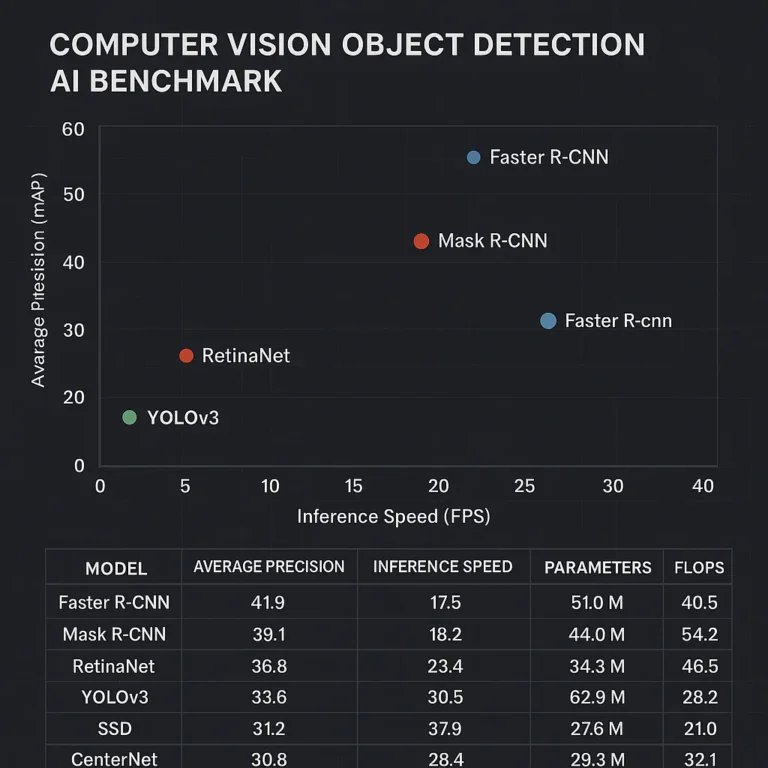
No detector family wins every contest. Compare implementations, not just names: “YOLO,” “Faster R-CNN,” and “DETR” each refer to families with multiple sizes, versions, training recipes, and deployment optimizations.
| Family or example | Broad approach | Often considered for | What to verify |
|---|---|---|---|
| Faster R-CNN | Two-stage region proposal and refinement. | Detailed detection pipelines and accuracy-focused comparisons. | Latency, memory use, and performance on your target image sizes. |
| YOLO | One-stage detection family. | Real-time and general-purpose applications. | Version, model size, runtime, input resolution, and post-processing. |
| SSD | One-stage detector using predictions across feature maps. | Efficient detection baselines and embedded-oriented comparisons. | Small-object performance and current implementation support. |
| RetinaNet | One-stage detector designed to address foreground-background imbalance. | Comparisons where class imbalance is a concern. | Training recipe, inference cost, and dataset-specific results. |
| DETR | Transformer-based detection approach using object queries. | Attention-based architectures and simplified detection pipelines. | Convergence, model variant, latency, and deployment constraints. |
Faster R-CNN and other two-stage detectors
Two-stage detectors first generate candidate regions, then classify and refine them. The original Faster R-CNN paper introduced a region proposal network that shares convolutional features with the detector.
Potential strengths include strong localization and flexible region-based processing. Trade-offs can include added computation and more complex inference. Do not assume every two-stage model is slow or every one-stage model is fast: implementation and hardware can overturn broad expectations.
YOLO and other one-stage detectors
YOLO-family models predict object locations and classes in a one-stage pipeline. They are popular for real-time applications, but comparisons must specify the exact version and configuration.
The featured YOLOv8 comparison video, “YOLOv8 Comparison with Latest YOLO models” by Pamudu Ranasinghe, shows examples under daylight, low light, blur, and fast-moving-object conditions. It’s a useful visual companion because it highlights the kind of conditions that a single benchmark score can obscure. A short video demonstration is illustrative, not a substitute for a controlled evaluation on your own data.
For current model details, consult the official Ultralytics documentation. The model name alone doesn’t tell you the input size, hardware, confidence threshold, or dataset behind a particular performance claim.
SSD, RetinaNet, and efficient detectors
SSD predicts detections across multiple feature maps. RetinaNet introduced focal loss to address class imbalance between foreground objects and the many background locations in dense detection.
These architectures are useful points of comparison, particularly when you want to understand how one-stage designs handle different scales and class imbalance. For present-day deployment decisions, benchmark maintained implementations and supported runtimes rather than relying only on historic paper results.
DETR and transformer-based object detection
DETR reframed detection as a set-prediction problem using a transformer encoder–decoder and object queries. Later transformer-based detector families have explored improvements to training efficiency and detection quality.
Transformer-based does not mean automatically more accurate, faster, or larger. The practical results depend on the variant, training recipe, data scale, and hardware. Compare against strong convolutional baselines using the same evaluation and deployment conditions.
🏭 Production Deployment and Ongoing Monitoring
A detector does not become reliable merely because it passed a test once. Production brings new cameras, changing environments, software updates, and occasional surprises that no benchmark split can fully predict.
Edge, cloud, and embedded deployment
| Deployment pattern | Potential benefits | Common trade-offs |
|---|---|---|
| Edge or on-device | Low network dependence, local processing, and potential privacy advantages. | Device limits, thermal constraints, and model-update complexity. |
| Cloud inference | Centralized deployment and access to scalable compute. | Network delay, connectivity dependence, and data-transfer considerations. |
| Embedded system | Direct integration with a specialized device or sensor. | Strict power, memory, and runtime constraints. |
| Hybrid | Local filtering plus centralized analysis or review. | More components to monitor and coordinate. |
Choose based on the whole system: latency, privacy, connectivity, update procedures, and failure modes. A detector that runs beautifully in a notebook but cannot be updated safely is not finished.
Monitor latency, accuracy, and data drift
Monitor operational signals such as:
- p50, p95, and p99 latency
- Throughput and dropped frames
- Confidence-score distributions
- Detections per class and per camera
- Input resolution and image quality
- Human-reviewed precision or miss rates, where available
- Changes in sensor, software, and environment
A shift in detection counts does not automatically prove the model has degraded; the real-world scene may have changed. Combine model telemetry with labeled samples and operational context before retraining.
Set task-specific acceptance criteria
Define pass/fail criteria before deployment. Include:
- Minimum recall for critical classes
- Maximum false-alarm rate
- Localization requirements at stated IoU thresholds
- Latency and throughput targets on target hardware
- Performance under specified conditions
- A process for reviewing failures and rolling back changes
Competitive advantage comes from reliable decisions, not a leaderboard screenshot. A detector that helps your team act faster, reduces costly inspection effort, or improves service consistency can be more valuable than a marginal benchmark gain. But only if its performance is measured against the outcome the business actually cares about.