Support our educational content for free when you purchase through links on our site. Learn more
15 Computer Vision KPIs That Reveal Model Performance 🔍

What are the key performance indicators for evaluating computer vision models? The right KPIs depend on the task: use precision, recall, and F1 for classification; IoU and mAP for object detection; and IoU or Dice for segmentation. Then check latency, robustness, and performance on representative data—because a strong benchmark score alone doesn’t guarantee a model will work in production.
We’ve seen how one deceptively high accuracy score can hide a serious miss: when defective products are rare, a model can label nearly everything “normal” and still look successful on paper. The useful question isn’t simply “How high is the score?” It’s “Which errors does this score reveal—and which might it conceal?”
Key Takeaways
- Match KPIs to the vision task: classification, detection, segmentation, and regression need different metrics.
- Look beyond accuracy: use precision, recall, F1, confusion matrices, IoU, mAP, or MAE as appropriate.
- Connect metrics to error costs: prioritize finding more true cases or reducing false alarms based on the application.
- Check data quality and test-set independence: leakage, weak labels, or unrepresentative data can make results misleading.
- Evaluate production readiness: measure latency, throughput, calibration, robustness, and performance across relevant conditions.
- Treat one score as a clue, not a verdict: inspect class-level results and real failure examples before deciding whether a model is ready.
Table of Contents
- ⚡️ Quick Tips and Facts
- 🧭 What Computer Vision Model Evaluation Really Measures
- How evaluation differs across vision tasks
- Offline metrics versus real-world performance
- 📚 Background: How Computer Vision Benchmarks Evolved
- 📊 15 Key Performance Indicators for Computer Vision Models
- 1. Accuracy and balanced accuracy
- 2. Precision: how many predictions are correct?
- 3. Recall: how many real objects or cases are found?
- 4. F1 score and F-beta score
- 5. Confusion matrix and class-wise errors
- 6. Intersection over Union (IoU)
- 7. Mean Average Precision (mAP)
- 8. Dice coefficient and segmentation overlap
- 9. Mean Absolute Error (MAE) and regression error
- 10. Root Mean Squared Error (RMSE)
- 11. ROC curve and Area Under the Curve (AUC)
- 12. Precision–Recall curve and Average Precision
- 13. Calibration and confidence scores
- 14. Inference latency, throughput, and memory use
- 15. Robustness, fairness, and safety indicators
- 🎯 Choosing Metrics for Each Computer Vision Task
- Image classification
- Object detection and tracking
- Semantic and instance segmentation
- Keypoint detection and pose estimation
- Image restoration, depth, and visual regression
- 🧪 Computer Vision Model Evaluation Techniques
- Build a reliable training, validation, and test split
- Prevent data leakage and duplicate-image contamination
- Use cross-validation when data is limited
- Set decision thresholds for the real use case
- Run error analysis and inspect difficult examples
- 🗂️ Dataset Considerations That Can Make or Break Results
- Label quality, annotation guidelines, and inter-annotator agreement
- Class imbalance and rare-event evaluation
- Data augmentation and distribution shift
- Representative data, subgroups, and edge cases
- 🏁 Benchmarking and Comparing Computer Vision Models
- Why benchmark design matters
- Popular public computer vision datasets
- Compare models using consistent metrics and conditions
- Report uncertainty, confidence intervals, and statistical significance
- Read leaderboard results without being fooled
- ⚖️ How to Balance Accuracy, Speed, Cost, and Risk
- Metric trade-offs and business requirements
- Evaluate models on edge devices and production hardware
- Set acceptance criteria and deployment guardrails
- 🚀 Monitoring Computer Vision Models After Deployment
- Data drift, concept drift, and changing environments
- Track live performance when labels arrive late
- Retraining triggers and ongoing evaluation
- 🛠️ A Practical Computer Vision Evaluation Workflow
- ❓ Frequently Asked Questions
- Which metric is best for evaluating a computer vision model?
- Is accuracy enough to evaluate an image classifier?
- What is a good IoU or mAP score?
- How do you evaluate a model with imbalanced classes?
- How often should a deployed vision model be evaluated?
- ✅ Conclusion
- 🔗 Recommended Links
- 📖 Reference Links
⚡️ Quick Tips and Facts
Computer vision KPIs are task-specific. Accuracy alone can flatter a model that misses the cases you care about most. Start by asking what the model must detect, what counts as a costly mistake, and where it will run.
Our team’s first stop is this guide to computer vision benchmarks: a score is only meaningful when you know the dataset, metric, and evaluation protocol behind it.
| Quick check | What to do |
|---|---|
| ✅ Match metric to task | Use classification metrics for classification, IoU and mAP for detection, and mIoU or Dice for segmentation. |
| ✅ Match metric to error cost | Prioritize recall when missing a positive is costly; precision when false alarms are costly. |
| ✅ Inspect more than one score | Pair headline metrics with per-class results, a confusion matrix, and examples of errors. |
| ✅ Test on unseen, representative data | Keep training, validation, and test sets distinct. Never use training performance as proof of generalization. |
| ✅ Check deployment behavior | Measure latency, throughput, memory, and performance under real camera, lighting, and hardware conditions. |
| ❌ Don’t trust accuracy by itself | If defects occur in only 2% of products, a model that always predicts “no defect” can achieve 98% accuracy while finding zero defects. |
Fast metric map: Classification → precision, recall, F1, and confusion matrix. Detection → IoU, AP, and mAP. Segmentation → mIoU and Dice. Regression → MAE, RMSE, and R². Production → add latency, reliability, and drift monitoring.
🧭 What Computer Vision Model Evaluation Really Measures
Computer vision model evaluation measures how well a model performs a defined task on data it did not simply memorize. That sounds tidy. In practice, “performs well” might mean correctly classifying an image, finding every safety helmet, outlining a tumor, estimating depth, or doing all of that before a conveyor belt carries the product away.
The Wapice evaluation guide puts it neatly: “A single number rarely tells the full story.” We agree. A model can post a strong aggregate score and still fail on small objects, rare classes, nighttime footage, or a particular camera angle.
How evaluation differs across vision tasks
| Task | Model output | Useful evaluation measures |
|---|---|---|
| Image classification | One or more labels for an image | Precision, recall, F1, accuracy, confusion matrix, ROC-AUC or PR-AUC |
| Object detection | Class labels and bounding boxes | IoU, precision, recall, AP, mAP |
| Semantic segmentation | A class label for each pixel | Class-wise IoU, mIoU, Dice, pixel accuracy |
| Instance segmentation | Separate masks for individual objects | Mask IoU, mask AP, detection-style precision and recall |
| Keypoint or pose estimation | Coordinates for landmarks or joints | OKS, PCK, mean keypoint error |
| Image regression | Continuous values, such as depth or defect size | MAE, RMSE, R²; task-specific errors |
| Image restoration | Reconstructed or enhanced image | PSNR, SSIM, perceptual metrics, and human review |
The metric must describe the actual output. For instance, pixel accuracy may look excellent in a road-scene segmentation task because most pixels are road or sky, even while the model misses pedestrians. CO’s evaluation tools use task-specific measures for detection and segmentation rather than pretending one generic score fits everything.
Offline metrics versus real-world performance
Offline evaluation answers, “How did this model perform on this labeled dataset?” Production evaluation asks, “Does it keep doing the job under the conditions people actually encounter?”
Those questions can diverge because of:
- Distribution shift: new locations, cameras, seasons, lighting, or product designs.
- Operational constraints: inference speed, connectivity, memory, and uptime.
- Human workflow: how many predictions require review and how easily staff can correct errors.
- Changing error costs: a false alarm may be tolerable during testing but disruptive at scale.
For broader deployment context, see our coverage of AI Business Applications and AI Infrastructure. A lab score is a starting point, not a production warranty. 🔍
📚 Background: How Computer Vision Benchmarks Evolved
Early computer vision benchmarks often focused on narrow tasks and fixed datasets. As datasets grew and models began producing richer outputs, evaluation expanded from simple classification accuracy to measures for localization, segmentation, confidence, and computational cost.
A few benchmarks helped standardize comparisons:
- ImageNet became a major large-scale image-classification benchmark.
- PASCAL VOC popularized object-detection evaluation with an IoU-based matching rule.
- CO broadened evaluation across object detection, instance segmentation, keypoints, and other tasks.
- Cityscapes supports semantic understanding of urban street scenes.
Standardized benchmarks make results easier to compare, but they do not automatically make a benchmark representative of your application. A model tested on sunny city streets may be a poor fit for a dim warehouse. Benchmark performance is a useful compass; your own data tells you whether the destination is right.
📊 15 Key Performance Indicators for Computer Vision Models
No single KPI wins every job. As Encord explains, “Each metric has its own set of strengths and weaknesses.” The practical move is to combine a primary success metric with diagnostics that explain why the score moved.
1. Accuracy and balanced accuracy
Accuracy is the fraction of predictions that are correct:
[
\text{Accuracy} = \frac{TP + TN}{TP + TN + FP + FN}
]
It is intuitive and useful when classes are reasonably balanced and false positives and false negatives have similar consequences.
Balanced accuracy averages recall across classes, giving each class equal weight. It is often more informative when one class dominates the dataset.
Watch out: on a dataset with 98% normal products and 2% defective products, predicting “normal” every time gives 98% accuracy and zero defect detection. Accuracy is not lying; it is answering a question you may not care about.
2. Precision: how many predictions are correct?
Precision measures the share of positive predictions that are true positives:
[
\text{Precision} = \frac{TP}{TP + FP}
]
Use precision when false alarms are costly. In manufacturing, for example, high precision can reduce unnecessary manual inspections and rejected products.
A precision score tells you little about cases the model failed to flag. Pair it with recall, especially when missed objects or defects matter.
3. Recall: how many real objects or cases are found?
Recall, also called sensitivity or true positive rate, measures the share of actual positives detected:
[
\text{Recall} = \frac{TP}{TP + FN}
]
Recall matters when false negatives are expensive: missed tumors, undetected safety hazards, or defects that reach customers.
High recall can bring more false positives, so plan for the review workload. In a medical workflow, a model that flags extra scans for clinician review may be preferable to one that quietly misses a concerning region.
4. F1 score and F-beta score
The F1 score is the harmonic mean of precision and recall:
[
F1 = 2 \times \frac{\text{Precision} \times \text{Recall}}{\text{Precision} + \text{Recall}}
]
It is useful when both false positives and false negatives matter and neither should dominate. But F1 gives precision and recall equal weight, which may not reflect the application.
The F-beta score lets you choose the balance:
- F2 emphasizes recall.
- F0.5 emphasizes precision.
Choose the weighting based on the cost of errors, not because one version sounds more impressive.
5. Confusion matrix and class-wise errors
A confusion matrix counts correct and incorrect predictions by class. In binary classification, it summarizes:
| Actual / Predicted | Positive | Negative |
|---|---|---|
| Positive | True positive (TP) | False negative (FN) |
| Negative | False positive (FP) | True negative (TN) |
For multi-class classification, each row and column represents a class. The matrix can reveal that a model frequently mistakes “cracked” for “scratched,” even if its overall accuracy looks respectable.
Use a confusion matrix alongside per-class precision and recall. scikit-learn’s documentation explains how to compute and interpret standard classification metrics.
6. Intersection over Union (IoU)
Intersection over Union measures how much a predicted region overlaps the ground-truth region:
[
IoU = \frac{\text{Area of Intersection}}{\text{Area of Union}}
]
IoU ranges from 0 (no overlap) to 1 (perfect overlap). It evaluates localization quality for bounding boxes and masks.
A prediction may correctly identify a dog but draw a sloppy box around half the image. Classification is right; localization is not. IoU makes that distinction visible. The IoU threshold used to count a detection as correct depends on the evaluation protocol: a loser threshold rewards finding the object, while a stricter one rewards tighter localization.
7. Mean Average Precision (mAP)
Average Precision (AP) summarizes a class’s precision–recall trade-off across confidence thresholds. Mean Average Precision (mAP) averages AP across classes, and in some protocols across multiple IoU thresholds.
The label “mAP” can refer to different calculations. For example, a benchmark may report AP at one IoU threshold, while another averages AP over IoUs from 0.50 to 0.95. Always report the dataset, IoU thresholds, class averaging, and matching protocol. Without those details, two mAP scores may not be comparable.
8. Dice coefficient and segmentation overlap
The Dice coefficient measures overlap between predicted and reference masks:
[
Dice = \frac{2|P \cap G|}{|P| + |G|}
]
Here, (P) is the predicted region and (G) is the ground-truth region. Dice ranges from 0 to 1, with higher values indicating better overlap.
Dice is closely related to F1 and is commonly used for segmentation, including medical imaging. It can be more informative than pixel accuracy when the object of interest occupies only a small fraction of an image. For fuller diagnostics, report class-wise Dice or IoU rather than only a global average.
9. Mean Absolute Error (MAE) and regression error
For a model predicting a continuous value—such as object size, depth, or defect severity—MAE is the average absolute difference between prediction and ground truth:
[
MAE = \frac{1}{n}\sum_{i=1}^{n} |y_i – \hat{y}_i|
]
MAE is expressed in the target’s units and treats errors linearly. If depth is measured in meters, the MAE is also in meters. It is generally less sensitive to large outliers than squared-error metrics.
10. Root Mean Squared Error (RMSE)
RMSE is the square root of mean squared error:
[
RMSE = \sqrt{\frac{1}{n}\sum_{i=1}^{n}(y_i-\hat{y}_i)^2}
]
Because errors are squared before averaging, RMSE penalizes large misses more heavily than MAE. That is useful when large errors are especially damaging, but it can also let a few outliers dominate the score.
Report MAE and RMSE together when both typical error and large-error behavior matter.
11. ROC curve and Area Under the Curve (AUC)
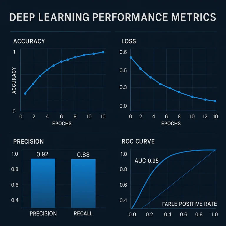
A Receiver Operating Characteristic (ROC) curve plots true positive rate against false positive rate as the classification threshold changes. ROC-AUC summarizes how well the model ranks positive examples above negative ones across thresholds.
ROC-AUC can help compare classifiers when the operating threshold has not yet been chosen. It does not tell you which threshold to deploy, nor does a high AUC guarantee useful precision when positive examples are rare.
12. Precision–Recall curve and Average Precision
A Precision–Recall (PR) curve shows how precision changes as recall changes across thresholds. It is especially useful when the positive class is rare because it focuses attention on positive predictions.
Average Precision summarizes the PR curve. For imbalanced detection or classification, PR analysis often reveals weaknesses that ROC-AUC can make less obvious. Compare it with the positive-class prevalence and a baseline; a score has no useful context on its own.
13. Calibration and confidence scores
A model is calibrated when its confidence scores match observed correctness rates. If predictions assigned 80% confidence are correct about 80% of the time across comparable examples, the model is well calibrated in that range.
Calibration matters when confidence controls:
- Whether a prediction is automatically accepted.
- Whether an image is sent to human review.
- Whether a system raises an alert.
Use reliability diagrams or proper scoring rules such as the Brier score to investigate calibration. A confidence score is not automatically a probability you can trust.
14. Inference latency, throughput, and memory use
A model can be accurate and still miss its business target if it is too slow or too resource-intensive.
| Operational KPI | What it tells you | Why it matters |
|---|---|---|
| Latency | Time to process one image or frame | Important for real-time inspection, robotics, and interactive applications |
| Throughput | Images or frames processed per second | Important for high-volume video and batch jobs |
| Memory use | GPU, CPU, and accelerator memory required | Determines whether the model fits target hardware |
| Availability | How reliably the service is running | Affects operational continuity |
| Cost per inference | Compute used per prediction at deployment scale | Helps compare system-level efficiency |
Measure on the hardware and input sizes you plan to deploy. A benchmark on a high-end GPU will not predict how the model behaves on an edge device.
15. Robustness, fairness, and safety indicators
Average performance can hide fragile or uneven behavior. Test performance across relevant subgroups and conditions: lighting, weather, camera type, geography, skin tone where applicable, age, object size, and oclusion.
Useful additional indicators include:
- Worst-group performance: the weakest result across important subgroups.
- Coruption robustness: performance under blur, noise, compression, or exposure changes.
- Out-of-distribution behavior: whether unfamiliar inputs trigger safe handling or confident mistakes.
- Human-review rate: the share of predictions escalated for review.
- Failure severity: how harmful the error is, not just how often it occurs.
The right set depends on the application. A warehouse counter and a clinical imaging tool should not have identical risk thresholds. For more deployment-related discussion, browse our AI News coverage.
🎯 Choosing Metrics for Each Computer Vision Task
The most useful KPI is the one that reflects the model’s job and the cost of getting it wrong. Here is a practical task-by-task map.
| Computer vision task | Primary metrics | Helpful diagnostics |
|---|---|---|
| Image classification | Per-class precision, recall, F1; balanced accuracy | Confusion matrix, ROC-AUC, PR-AUC, calibration |
| Object detection | AP and mAP at stated IoU thresholds | Per-class recall, box IoU, small-object performance |
| Semantic segmentation | Class-wise IoU, mIoU, Dice | Pixel accuracy, boundary quality, per-class error maps |
| Instance segmentation | Mask AP, mask IoU, mAP | Detection recall, mask quality by object size |
| Pose estimation | OKS, PCK, mean keypoint error | Per-joint errors, oclusion-specific performance |
| Regression or depth estimation | MAE, RMSE, R² | Residual plots, error by distance or range |
Image classification
For classification, start with per-class precision and recall, not only aggregate accuracy. Add F1 when you want a compact balance of the two, and inspect the confusion matrix to see which classes the model confuses.
For rare positive classes, include PR-AUC and choose a threshold based on the cost of false alarms versus misses. In a consumer-photo classifier, occasional false positives may be harmless. In quality control, a missed defect can be costly.
Object detection and tracking
For object detection, report mAP with its IoU protocol, plus per-class recall and performance by object size. Average performance can conceal trouble finding small, partially ocluded, or distant objects.
For tracking, detection scores are not enough. Add measures of identity consistency and tracking accuracy, such as HOTA, MOTA, or IDF1, depending on the tracking evaluation protocol. A detector that finds every person but swaps identities constantly is not a good tracker.
Semantic and instance segmentation
For semantic segmentation, use class-wise IoU and mIoU to assess region overlap. Add Dice where overlap on small target regions matters, and pixel accuracy only as a supporting measure.
For instance segmentation, the system must both identify each object and outline its mask. Use a benchmark that evaluates mask quality and detection matching, such as the CO evaluation protocol.
Keypoint detection and pose estimation
Keypoint models predict coordinates for landmarks, joints, or other points. Percentage of Correct Keypoints (PCK) measures the fraction of predicted points within a specified distance of the reference. Object Keypoint Similarity (OKS) accounts for localization error, object scale, and keypoint visibility in common pose benchmarks.
Report per-keypoint performance: a strong average can hide weak estimates for wrists, ankles, or other difficult landmarks.
Image restoration, depth, and visual regression
For depth estimation or other continuous outputs, use MAE and RMSE, then break errors down by range or scene type. For image restoration, PSNR and SSIM are common, but pixel similarity does not always match perceived image quality. A visually smooth result may erase details a downstream system needs.
When human perception matters, combine numerical scores with a structured human review. For broader automation context, see AI Automation Workflows.
🧪 Computer Vision Model Evaluation Techniques
A credible evaluation is a process, not a single model.evaluate() call. Here’s the workflow our team uses to avoid producing a polished score with a shaky foundation.
Build a reliable training, validation, and test split
- Define the unit of separation. If multiple images come from the same video, person, product, or site, keep related images in the same split.
- Create the training split. Use this data to fit model parameters.
- Create the validation split. Use it to select checkpoints, tune hyperparameters, and choose thresholds.
- Reserve the test split. Use it for final evaluation after major decisions are complete.
- Preserve relevant diversity. Ensure each split reflects important classes, locations, cameras, and conditions.
- Document the split. Record dataset versions, sampling rules, and any exclusions so the result can be reproduced.
Common split ratios are only starting points. A large, diverse dataset may support a small test fraction; a small dataset may benefit from grouped cross-validation. The split must fit the data structure, not a rule of thumb.
Prevent data leakage and duplicate-image contamination
Data leakage happens when information from validation or test data influences training or model selection. It can make a model look far better than it will perform on genuinely new data.
Common traps include:
- Near-duplicate frames from the same video appearing in both training and test sets.
- Images of the same patient or product split across datasets.
- Preprocessing or feature selection informed by test labels.
- Repeatedly tuning against the test set until it is no longer independent.
Use grouped splits, duplicate detection, and strict test-set access controls. The scikit-learn cross-validation guide explains why appropriate splitting matters.
Use cross-validation when data is limited
In k-fold cross-validation, the dataset is divided into (k) folds. The model trains on (k-1) folds and validates on the remaining fold, repeating until each fold has served as validation data.
Cross-validation can produce a more stable estimate when data is limited. But it does not fix leakage, and it may be inappropriate if samples are correlated. Grouped or time-based cross-validation is often more suitable for video, medical, or production data.
Set decision thresholds for the real use case
A classifier’s threshold controls how confident it must before predicting a positive. Lowering the threshold often increases recall and false positives; raising it often improves precision while missing more positives.
- Choose the error type that matters most.
- Plot precision and recall across thresholds.
- Estimate the human-review or operational cost at each threshold.
- Select a threshold on validation data.
- Freeze it before the final test.
- Revisit it when the data or business requirements change.
A threshold chosen from the test set contaminates the final evaluation. Resist the temptation; the test set is the referee, not the coach.
Run error analysis and inspect difficult examples
After calculating metrics, review representative failures. Sort examples by confidence, object size, class, lighting, oclusion, or error severity. Ask:
- Is the label wrong or ambiguous?
- Is the failure concentrated in one subgroup or capture condition?
- Did the model miss the object, misclassify it, or localize it poorly?
- Would more representative data address the issue?
- Is the metric counting the error in a way that matches the application?
The first video makes a useful practical point: a model does not need to be perfect to be useful, but the evaluation should focus on the right metric. Its examples also highlight how low recall can matter more than strong overall accuracy in cancer detection, and how small-object detection may need targeted fixes such as SAHI.
🗂️ Dataset Considerations That Can Make or Break Results
A metric can be calculated perfectly on a dataset that is poorly labeled, unrepresentative, or contaminated. Dataset quality is not background housekeeping; it is part of the evaluation itself.
Label quality, annotation guidelines, and inter-annotator agreement
Review annotation instructions before interpreting model errors. If two annotators disagree about what counts as a defect, a model may appear wrong when the ground truth is inconsistent.
Track:
- Label agreement: how consistently annotators apply the rules.
- Boundary consistency: whether object outlines are drawn to a consistent standard.
- Ambiguity rate: how often an example cannot be labeled confidently.
- Correction rate: how often expert review changes labels.
For segmentation and detection, small differences in boundaries can change IoU or Dice. A model score should be interpreted in light of the quality and consistency of its reference annotations.
Class imbalance and rare-event evaluation
When some classes are rare, overall accuracy and micro-averaged scores can be dominated by common examples. Report per-class precision, recall, and support (the number of examples for each class). Macro-averaging gives classes equal weight; micro-averaging pools individual predictions and emphasizes frequent classes.
Training methods such as class weighting or oversampling can help, but they do not replace an evaluation set that reflects real-world prevalence. Avoid synthetic examples or resampling in the test set unless the goal is specifically to evaluate on that altered distribution.
Data augmentation and distribution shift
Augmentation can expose a model to useful variation, such as mild rotation, scale changes, or color shifts. But augmentation should represent plausible conditions for the application. A transformation that improves a benchmark score may teach the model to ignore a visual feature that matters in production.
Test separately across:
- Day and night, or bright and dim lighting.
- Different camera sensors and image resolutions.
- Weather, blur, compression, and oclusion.
- New products, locations, or backgrounds.
- Changes in object size and viewing angle.
Representative data, subgroups, and edge cases
Build evaluation slices for the conditions that matter. For example, a retail shelf model may need separate results for crowded shelves, reflective packaging, partially hidden items, and camera distance.
A useful test set is not merely large; it is representative of deployment and rich in meaningful edge cases. Document how each slice was chosen, and avoid reporting subgroup results without enough examples to interpret them responsibly.
🏁 Benchmarking and Comparing Computer Vision Models
Benchmarks help answer “Which model performed better under the same conditions?” They do not automatically answer “Which model should we deploy?”
Why benchmark design matters
A fair comparison requires the same:
- Dataset and data split.
- Preprocessing and input resolution.
- Metric definitions and thresholds.
- Hardware and inference settings.
- Annotation rules and exclusion criteria.
Otherwise, a score may reflect different evaluation conditions rather than a better model. This is why a benchmark report should include details, not just a leaderboard rank.
Popular public computer vision datasets
| Dataset | Common use | Useful caution |
|---|---|---|
| ImageNet | Large-scale image classification | Label taxonomy and images may not match a specialized deployment domain |
| CO | Object detection, segmentation, keypoints | Results depend on the task and evaluation protocol |
| PASCAL VOC | Classification and object detection | A useful established benchmark, but smaller and narrower than many deployment datasets |
| CIFAR-10 and CIFAR-100 | Small-image classification research | Low-resolution images limit conclusions about high-resolution production imagery |
| MNIST | Handwritten digit recognition | Too simple to stand in for general-purpose visual recognition |
| ADE20K | Scene parsing and segmentation | Check class definitions and scene coverage against the target use case |
| Cityscapes | Urban-scene semantic segmentation | Focused on driving scenes; not a general indoor or industrial benchmark |
| Labeled Faces in the Wild (LFW) | Face verification research | Benchmark scores do not establish suitability or fairness for every use |
Public datasets are excellent for reproducibility and initial comparison. They cannot replace a representative, independently labeled test set from the intended application.
Compare models using consistent metrics and conditions
For each candidate, report:
- The primary task metric and its exact definition.
- Per-class results and sample counts.
- Performance by important subgroup or operating condition.
- Latency, throughput, and memory on target hardware.
- Calibration and threshold behavior if confidence affects decisions.
- Known limitations and the benchmark version.
Tools such as pycocotools, TorchMetrics, MLflow, and Weights & Biases can help standardize evaluation and track experiments. Choose tools that fit your stack and governance needs.
Report uncertainty, confidence intervals, and statistical significance
A metric is an estimate from a finite sample. If two models differ by a small amount, that gap may not be meaningful.
Use confidence intervals or bootstrap resampling where appropriate, and report the number of images, objects, or patients behind each result. For correlated images—such as adjacent video frames—resample at the group level rather than treating every frame as independent.
The practical question is not only “Is model A’s score higher?” It is also “Is the improvement consistent enough to matter?”
Read leaderboard results without being fooled
Before trusting a leaderboard score, check:
- The exact dataset version and hidden-test rules.
- Whether evaluation averages across classes or examples.
- Whether the result uses one threshold or several.
- The model’s input resolution and inference setup.
- Whether test data may have influenced model development.
- Whether the benchmark resembles your production conditions.
A leaderboard is a useful snapshot, not a deployment certificate. 🏁
⚖️ How to Balance Accuracy, Speed, Cost, and Risk
Computer vision systems are products as well as models. A small accuracy gain may not justify a large increase inference time, review burden, or system complexity.
Metric trade-offs and business requirements
Write down the consequences of each error before choosing the primary KPI.
| Application example | Mistake to control | Metrics to emphasize |
|---|---|---|
| Medical image triage | Missed high-risk finding | Recall, sensitivity, calibration; specialist review |
| Manufacturing inspection | Defect passes undetected | Recall by defect type, false-negative rate, defect-size analysis |
| Retail inventory | Incorrect item count | Counting error, detection recall, performance by oclusion |
| Content moderation | Harmful content missed or harmless content flagged | Per-class precision and recall, subgroup analysis, review rate |
| Real-time robotics | Late or missed perception | Detection quality, latency, throughput, robustness |
Business requirements should become measurable acceptance criteria. “The model should be reliable” is a nice sentiment; “recall for critical defects must exceed the agreed threshold on representative test data” is something a team can actually verify.
Evaluate models on edge devices and production hardware
If the model will run on a device rather than a cloud server, measure the complete pipeline on that hardware. Include image decoding, resizing, inference, post-processing, network time, and output handling.
Evaluate:
- Median and tail latency, not only average latency.
- Throughput at realistic batch sizes.
- Memory use and thermal behavior.
- Performance after quantization or pruning.
- Connectivity loss and recovery, where relevant.
For a broader look at compute and deployment trade-offs, visit AI Infrastructure. A model that runs smoothly in a notebook may behave very differently in a warm enclosure beside a production line.
Set acceptance criteria and deployment guardrails
Before deployment, define minimum thresholds for task quality, subgroup performance, latency, and reliability. Add guardrails for:
- Low-confidence predictions.
- Out-of-distribution or corrupted inputs.
- Suden shifts input data.
- Human escalation and override.
- Rollback if a new model regresses.
These checks help turn evaluation from a one-time report into an operational safety net.
🚀 Monitoring Computer Vision Models After Deployment
A model’s inputs can change after launch, even if its code does not. New cameras, lighting, products, or user behavior can gradually weaken performance.
Data drift, concept drift, and changing environments
Data drift means the input distribution changes. Concept drift means the relationship between inputs and the correct output changes. For example, a new package design may alter the appearance of a product; a revised quality standard may change what counts as a defect.
Monitor input characteristics and prediction patterns, then compare them with labeled outcomes when available. Drift is a warning signal, not proof that the model is failing. Confirm it with task metrics and representative review.
Track live performance when labels arrive late
Some applications receive labels only after a human review, customer report, or delayed quality inspection. In the meantime, monitor proxy signals:
- Prediction confidence and class distribution.
- Human override and escalation rates.
- Rework, rejection, or missed-inspection indicators.
- Latency, error rates, and service availability.
- Performance on a continuously labeled sample.
Proxies cannot replace ground-truth evaluation, but they can flag changes early enough to investigate.
Retraining triggers and ongoing evaluation
Retrain when there is evidence that the model no longer meets its acceptance criteria—not merely because the calendar says so. Before promoting a new version, run the same benchmark, test set, and subgroup checks used for the existing model.
Version the model, dataset, code, and evaluation configuration. Tools such as MLflow can help track experiments and artifacts; automated testing can flag regressions before release.
🛠️ A Practical Computer Vision Evaluation Workflow
Use this checklist to move from “the model seems good” to a defensible evaluation:
- Define the task and success criteria. Specify what the model predicts, who uses the output, and what errors cost.
- Choose a primary KPI and supporting diagnostics. For example, recall plus precision and confusion matrix for defect detection.
- Audit labels and dataset coverage. Check class balance, annotation quality, duplicates, and deployment relevance.
- Create leakage-resistant data splits. Group by patient, video, product, or site when examples are related.
- Freeze the evaluation protocol. Document metrics, thresholds, preprocessing, and exclusions.
- Evaluate a baseline. Compare against a simple or existing system; otherwise, a score has no practical reference point.
- Analyze class-wise and subgroup results. Find out who or what the aggregate average may be hiding.
- Inspect failure examples. Separate label problems, model errors, and application-design issues.
- Measure system performance. Test latency, throughput, memory, and reliability on intended hardware.
- Choose thresholds on validation data. Keep final test data independent.
- Report uncertainty and limitations. Include sample counts and confidence intervals where useful.
- Set production monitoring and rollback rules. Evaluation should continue after launch.
The first video reinforces two useful habits: do not evaluate final performance on training data, and focus on the metric tied to the application’s risk. That is the difference between a flattering demo and a trustworthy decision tool.
❓ Frequently Asked Questions
How do you choose the right performance metrics for a computer vision model?
Start with the model’s task and the cost of its mistakes. For classification, consider per-class precision, recall, F1, and a confusion matrix. For object detection, use AP or mAP with a stated IoU protocol. For segmentation, report class-wise IoU or Dice. For continuous outputs, use MAE or RMSE.
Then add the metrics needed to answer practical questions: Does the model miss rare cases? Is it calibrated? Does it run fast enough? Does it fail under certain conditions? We recommend a primary KPI plus complementary diagnostics, rather than one score standing alone.
How do computer vision KPIs affect real-world business outcomes?
KPIs connect model behavior to operational outcomes. Higher recall may reduce missed defects but increase inspections. Higher precision may reduce false alarms but allow more real defects to pass. Lower latency can enable real-time workflows, while better calibration can route uncertain cases to human review.
The business goal is not to maximize every metric at once. It is to choose a measurable trade-off that improves the workflow without creating unacceptable risk, cost, or workload.
What metrics best evaluate object detection and image classification models?
For object detection, use mAP or AP with clearly stated IoU thresholds, and include per-class recall and object-size analysis. IoU measures localization overlap; AP summarizes the precision–recall trade-off.
For image classification, use per-class precision, recall, F1, and a confusion matrix. Add PR-AUC for rare positive classes or ROC-AUC when threshold-independent ranking performance is useful. Report accuracy only with context about class balance and error costs.
How can businesses use computer vision KPIs to gain a competitive edge?
Use KPIs to identify the model and workflow combination that performs best under actual operating conditions. A business can use class-wise defect recall to reduce escapes, precision to limit unnecessary reviews, and latency to improve production throughput.
The advantage comes from turning evaluation into a feedback loop: measure performance, inspect failures, improve data or process design, and verify that changes help on independent test data. The strongest KPI strategy also tracks human review, reliability, and subgroup performance, not just a headline benchmark score.
Is accuracy enough to evaluate an image classifier?
Usually not. Accuracy can look high when one class dominates, even if the model never identifies the rare class you care about. Add per-class precision and recall, F1, and a confusion matrix. For highly imbalanced data, consider PR-AUC and report the class prevalence.
What is a good IoU or mAP score?
There is no universal “good” score. It depends on the task, object size, annotation quality, IoU thresholds, and the cost of localization errors. A benchmark score is comparable only when the dataset and evaluation protocol match.
Set an application-specific baseline and acceptance threshold, then test on representative data. A lower score on a difficult but relevant real-world dataset may be more useful than a higher score on an unrelated benchmark.
How do you evaluate a model with imbalanced classes?
Report class-wise precision, recall, F1, and the number of examples in each class. Use macro-averaged scores when each class deserves equal weight, and PR-AUC when rare positive examples matter. Inspect the confusion matrix and evaluate on data that reflects real deployment prevalence.
Resampling and class weighting may help training, but keep the final test set representative. Otherwise, the reported result may not describe real-world performance.
How often should a deployed vision model be evaluated?
Evaluate before every release, after significant changes to data or hardware, and periodically in production based on risk and label availability. High-risk systems may need continuous monitoring and frequent review; lower-risk workflows may use scheduled sampling.
Increase evaluation frequency after changes such as a new camera, location, product design, or operating procedure. Monitor drift and proxy signals, then validate suspected performance changes against labeled examples.