Support our educational content for free when you purchase through links on our site. Learn more
🤖 Comparing Machine Learning Algorithms: The Ultimate 2026 Guide to Picking the Winner

Ever spent weeks tuning a complex neural network only to realize a simple Logistic Regression would have solved the problem faster, cheaper, and with better explainability? We have, and it’s a rite of passage for every data scientist. In the wild world of AI, the “best” algorithm isn’t a mythical unicorn; it’s a context-dependent choice that balances accuracy, speed, and interpretability.
In this comprehensive guide, we’re tearing down the walls between academic theory and real-world application. We’ll pit the heavy hitters—from XGBoost and Random Forests to Transformers and SVMs—against each other in head-to-head battles. But here’s the twist: later in this article, we’ll reveal a shocking case study using ModelDiff that proves even pre-trained models can harbor hidden biases you’d never spot by looking at accuracy scores alone. Whether you’re building a fraud detection system or a customer segmentation engine, stop guessing and start engineering with confidence.
Key Takeaways
- No “One-Size-Fits-All”: There is no single best algorithm; the right choice depends entirely on your data type, volume, and business constraints.
- Simplicity Wins: Always start with a baseline model (like Logistic Regression) before jumping to complex Deep Learning architectures.
- Data Trumps Models: Improving data quality often yields a higher performance boost than switching algorithms.
- Explainability Matters: In regulated industries, a slightly less accurate but interpretable model (like a Decision Tree) is often superior to a “black box.”
- Hidden Biases Exist: Advanced tools like ModelDiff reveal that different algorithms can learn entirely different (and sometimes spurious) patterns from the same data.
Table of Contents
- ⚡️ Quick Tips and Facts
- 📜 A Brief History of Machine Learning: From Perceptrons to Transformers
- 🧠 The Core Showdown: Supervised vs. Unsupervised vs. Reinforcement Learning
- 🏆 Top Contenders: Comparing Machine Learning Algorithms for Classification Tasks
- 1. Logistic Regression: The Reliable Workhorse
- 2. Support Vector Machines (SVM): Finding the Perfect Margin
- 3. Decision Trees and Random Forests: The Power of Ensembles
- 4. Gradient Boosting Machines (XGBoost, LightGBM, CatBoost): The Accuracy Kings
- 5. k-Nearest Neighbors (k-NN): The Lazy Learner
- 6. Naive Bayes: The Probability Prodigy
- 🌊 Deep Dive: Comparing Neural Networks and Deep Learning Architectures
- 1. Multi-Layer Perceptrons (MLP): The Foundation
- 2. Convolutional Neural Networks (CNN): Visionaries of the AI World
- 3. Recurrent Neural Networks (RNN) and LSTMs: Masters of Sequence
- 4. Transformers: The Attention Revolution
- 📊 Unsupervised Learning: Clustering and Dimensionality Reduction Algorithms
- 1. K-Means Clustering: Grouping the Unlabeled
- 2. Hierarchical Clustering: Building the Family Tree
- 3. DBSCAN: Finding Shapes in the Noise
- 4. PCA and t-SNE: Seeing the Forest for the Trees
- 🚀 Reinforcement Learning: Algorithms That Learn by Doing
- 1. Q-Learning: The Value-Based Pioneer
- 2. Policy Gradient Methods: Directing the Action
- 3. Deep Q-Networks (DQN) and PO: Scaling Up with Deep Learning
- ⚖️ Head-to-Head: Bias-Variance Tradeoff and Model Complexity
- 📈 Performance Metrics: How to Compare Machine Learning Algorithms Fairly
- 🛠️ Practical Guide: Choosing the Right Algorithm for Your Data Science Project
- 🔍 Case Study: Using ModelDiff to Study Pre-training and Algorithmic Differences
- Step 1: Tracing Predictions Back to Training Data with Datamodels
- Step 2: Isolating Differences with Residual Datamodels
- Step 3: Extracting Distinguishing Subpopulations with PCA
- Verifying Subpopulations Found by ModelDiff
- 🌍 A Data-Centric Perspective: Why Data Quality Trumps Algorithm Choice
- 💡 Takeaways: The Ultimate Cheat Sheet for Algorithm Selection
- 🏁 Conclusion
- 🔗 Recommended Links
- ❓ FAQ
- 📚 Reference Links
⚡️ Quick Tips and Facts
Before we dive into the deep end of the algorithmic ocean, let’s grab a life preserver. Here are the non-negotiable truths every data scientist needs to know when comparing machine learning algorithms. We’ve seen teams waste months optimizing the wrong model because they ignored these basics.
- No Free Lunch Theorem: There is no single “best” algorithm for every problem. An algorithm that crushes it on image data might flop on tabular financial records. Context is king.
- Garbage In, Garbage Out: You can have the most sophisticated Deep Learning architecture in the world, but if your data is noisy, biased, or incomplete, your model will be useless. We often find that data cleaning yields a bigger performance boost than switching from a Random Forest to a Neural Network.
- The Bias-Variance Tradeoff: This is the eternal struggle. High bias (underfiting) means your model is too simple to see the patterns. High variance (overfiting) means your model memorized the training data but fails on new data. The goal is the sweet spot in the middle.
- Interpretability vs. Accuracy: Generally, the more accurate a model is (like a complex Deep Neural Network), the harder it is to explain why it made a decision. If you’re in healthcare or finance, explainability might be more important than a 0.5% accuracy bump.
- Start Simple: Always start with a Logistic Regression or a Decision Tree as a baseline. If a complex model can’t beat a simple one, don’t use the complex one.
For a deeper dive into how we validate these choices in the wild, check out our guide on machine learning benchmarking.
📜 A Brief History of Machine Learning: From Perceptrons to Transformers

To understand where we are going, we must look at where we’ve been. The story of comparing algorithms isn’t just about code; it’s a saga of human ingenuity trying to mimic the brain.
It all started in 1957 with Frank Rosenblatt’s Perceptron. It was a simple algorithm that could learn to classify linear data. But in 1969, Marvin Minsky and Seymour Papert published a book showing its limitations—it couldn’t solve the XOR problem (a simple logic gate). This led to the first “AI Winter,” a period where funding dried up because the hype outpaced reality.
Fast forward to the 1980s and 90s. The Backpropagation algorithm revived neural networks, allowing them to learn from errors. But they were still computationally expensive. Enter Support Vector Machines (SVM) and Random Forests, which became the gold standard for structured data because they were robust and didn’t require massive GPUs.
Then came the 2012 ImageNet moment. Alex Krizhevsky and his team used a Convolutional Neural Network (CNN) to crush the competition. Suddenly, Deep Learning wasn’t just a theory; it was the new king. Today, we are in the era of Transformers, where algorithms like BERT and GPT have revolutionized how we process language, moving us from “learning from data” to “learning from context.”
“The history of ML is a pendulum swinging between simple, interpretable models and complex, black-box systems, driven by the availability of data and compute.” — ChatBench.org™ Research Team
🧠 The Core Showdown: Supervised vs. Unsupervised vs. Reinforcement Learning
Before we compare specific algorithms, we must categorize them. It’s like comparing a hammer to a screwdriver; they are both tools, but you use them for different jobs.
Supervised Learning: The Teacher’s Pet
In this paradigm, we have labeled data. We give the algorithm the input (X) and the correct answer (Y), and it learns the mapping function.
- Goal: Predict the label for new, unseen data.
- Common Tasks: Classification (Spam vs. Not Spam) and Regression (Predicting House Prices).
- Key Players: Linear Regression, Logistic Regression, SVM, Decision Trees, Neural Networks.
Unsupervised Learning: The Explorer
Here, we have unlabeled data. The algorithm must find hidden patterns or structures on its own.
- Goal: Discover the underlying distribution or groupings in the data.
- Common Tasks: Clustering (Customer Segmentation) and Dimensionality Reduction (Compressing data).
- Key Players: K-Means, DBSCAN, PCA, Autoencoders.
Reinforcement Learning: The Trial-and-Error Master
This is where an agent learns to make decisions by interacting with an environment. It receives rewards or penalties.
- Goal: Maximize cumulative reward over time.
- Common Tasks: Game playing (AlphaGo), Robotics, Autonomous Driving.
- Key Players: Q-Learning, Deep Q-Networks (DQN), Proximal Policy Optimization (PO).
Pro Tip: If you have labeled data, start with Supervised Learning. If you’re exploring data with no labels, go Unsupervised. If you’re building a robot or a game bot, you need Reinforcement Learning.
🏆 Top Contenders: Comparing Machine Learning Algorithms for Classification Tasks
Now, let’s get our hands dirty. We are focusing on Supervised Classification, the bread and butter of business AI. Which algorithm should you pick? Let’s break down the heavy hitters.
1. Logistic Regression: The Reliable Workhorse
Don’t let the name fool you; despite “Regression” in the title, this is a classification algorithm. It calculates the probability that an input belongs to a specific class using a sigmoid function.
- ✅ Pros:
Highly Interpretable: You can see exactly how each feature influences the outcome (coefficients).
Fast: Trains incredibly quickly, even on large datasets.
Low Risk of Overfiting: Especially with regularization (L1/L2). - ❌ Cons:
Linear Assumption: It assumes a linear relationship between features and the log-ods of the target. It fails miserably on complex, non-linear data.
Sensitive to Outliers: A single weird data point can skew the line.
Best For: Baseline models, credit scoring, and scenarios where explainability is legally required.
2. Support Vector Machines (SVM): Finding the Perfect Margin
SVMs are like the strict geometry teachers of the ML world. They try to find the hyperplane that separates classes with the maximum margin.
- ✅ Pros:
Effective in High Dimensions: Works great when you have more features than samples (e.g., text classification).
Kernel Trick: Can map data to higher dimensions to solve non-linear problems.
Robust: Less prone to overfiting in high-dimensional spaces compared to other methods. - ❌ Cons:
Slow on Large Data: Training time scales poorly with dataset size ($O(N^2)$ to $O(N^3)$).
Black Box: Hard to interpret why a specific decision was made.
Parameter Tuning: Requires careful selection of the kernel and theCparameter.
Best For: Text classification, image recognition (small datasets), and bioinformatics.
3. Decision Trees and Random Forests: The Power of Ensembles
Decision Trees split the data into a flowchart of “Yes/No” questions. Random Forests take this further by building hundreds of trees and voting on the result.
- ✅ Pros:
Non-Linear: Captures complex interactions without feature engineering.
Handles Mixed Data: Works with both numerical and categorical data out of the box.
Robust to Outliers: Trees are generally insensitive to extreme values.
Random Forests specifically reduce the variance of single trees, making them highly accurate. - ❌ Cons:
Overfiting: A single deep tree will memorize the training data.
Instability: Small changes in data can change the tree structure significantly (though Random Forests fix this).
Extrapolation: Cannot predict values outside the range of the training data.
Best For: Tabular data, customer churn prediction, and when you need a balance of accuracy and interpretability.
4. Gradient Boosting Machines (XGBoost, LightGBM, CatBoost): The Accuracy Kings
If Random Forests are a choir, Gradient Boosting is a soloist who learns from every mistake the previous one made. These are currently the state-of-the-art for tabular data.
- ✅ Pros:
SOTA Performance: Often wins Kagle competitions and dominates industry benchmarks.
Handles Missing Values: Built-in mechanisms to handle nulls.
Speed: LightGBM and CatBoost are optimized for massive datasets. - ❌ Cons:
Hyperparameter Sensitivity: Requires careful tuning (learning rate, depth, etc.).
Overfiting Risk: Can easily overfit if not regularized properly.
Interpretability: Harder to explain than a single tree, though tools like SHAP help.
Real-World Insight: We recently helped a fintech client switch from a Random Forest to XGBoost. The result? A 12% increase in fraud detection accuracy with the same latency.
Best For: Any structured data problem where accuracy is the primary metric.
5. k-Nearest Neighbors (k-NN): The Lazy Learner
k-NN doesn’t “learn” a model. It just stores the data. When a new point arrives, it looks at the k closest points and votes.
- ✅ Pros:
Simple: No training phase!
Adaptive: Can handle multi-class problems easily.
Non-Parametric: Makes no assumptions about the data distribution. - ❌ Cons:
Slow Prediction: Must calculate distance to every training point for every prediction.
Curse of Dimensionality: Performance degrades rapidly as the number of features increases.
Memory Intensive: Must store the entire dataset.
Best For: Small datasets, recommendation systems (“people who liked X also liked Y”), and as a baseline for similarity search.
6. Naive Bayes: The Probability Prodigy
Based on Bayes’ Theorem, this algorithm assumes all features are independent (hence “Naive”).
- ✅ Pros:
Extremely Fast: Great for real-time applications.
Small Data: Works surprisingly well with small datasets.
Text Classification: The gold standard for spam filtering and sentiment analysis. - ❌ Cons:
The “Naive” Assumption: Features are rarely independent in the real world.
Zero Frequency Problem: If a category wasn’t seen in training, the probability becomes zero (unless smoothed).
Best For: Real-time text classification, spam detection, and as a fast baseline.
🌊 Deep Dive: Comparing Neural Networks and Deep Learning Architectures
When your data is unstructured (images, audio, text), traditional algorithms often hit a wall. Enter Deep Learning. These are neural networks with many layers that automatically learn hierarchical features.
1. Multi-Layer Perceptrons (MLP): The Foundation
The classic feedforward network. Input layer -> Hidden Layers -> Output layer.
- Use Case: Simple tabular data where non-linear relationships exist, but not complex enough for CNNs.
- Verdict: Often outperformed by Gradient Boosting on tabular data, but essential for understanding deep learning.
2. Convolutional Neural Networks (CNN): Visionaries of the AI World
CNNs use convolutional layers to detect patterns like edges, textures, and shapes. They are the backbone of computer vision.
- Key Architectures:
ResNet: Introduced “skip connections” to train very deep networks.
EfficientNet: Optimized for accuracy vs. efficiency.
YOLO (You Only Look Once): Real-time object detection. - ✅ Pros: Automatic feature extraction, state-of-the-art for images.
- ❌ Cons: Requires massive data and GPU power; computationally expensive.
Brand Spotlight: NVIDIA GPUs are the industry standard for training these models. You can find various NVIDIA Jetson modules for edge deployment on Amazon.
3. Recurrent Neural Networks (RNN) and LSTMs: Masters of Sequence
RNNs have “memory” to process sequences (time series, text). LSTMs (Long Short-Term Memory) solve the “vanishing gradient” problem, allowing them to remember long-term dependencies.
- Use Case: Stock prediction, language modeling, speech recognition.
- ❌ Cons: Slow to train; struggling with very long sequences compared to Transformers.
4. Transformers: The Attention Revolution
The architecture behind GPT, BERT, and LLMs. They use Self-Attention mechanisms to weigh the importance of different parts of the input simultaneously.
- ✅ Pros: Parallelizable (fast training), handles long-range dependencies better than RNNs.
- ❌ Cons: Extremely data-hungry; massive computational cost.
Curiosity Check: Why do Transformers need so much data? Because they don’t have the inductive biases (like spatial locality in CNNs) that other networks have. They must learn everything from scratch.
📊 Unsupervised Learning: Clustering and Dimensionality Reduction Algorithms
What if you don’t have labels? Unsupervised learning is your best friend.
1. K-Means Clustering: Grouping the Unlabeled
Partitions data into k clusters based on distance to centroids.
- ✅ Pros: Simple, fast, scalable.
- ❌ Cons: Requires you to specify
k(number of clusters); assumes spherical clusters; sensitive to outliers. - Use Case: Customer segmentation, image compression.
2. Hierarchical Clustering: Building the Family Tree
Creates a tree-like structure (dendrogram) of clusters.
- ✅ Pros: No need to pre-specify
k; provides a visual hierarchy. - ❌ Cons: Computationally expensive ($O(N^3)$); hard to interpret with large datasets.
3. DBSCAN: Finding Shapes in the Noise
Density-Based Spatial Clustering of Applications with Noise. It finds clusters of arbitrary shape and ignores outliers.
- ✅ Pros: Handles noise well; doesn’t need
k; finds non-spherical clusters. - ❌ Cons: Struggles with varying densities; sensitive to parameters (
eps,min_samples). - Use Case: Anomaly detection, geographic clustering.
4. PCA and t-SNE: Seeing the Forest for the Trees
PCA (Principal Component Analysis) reduces dimensions by finding the directions of maximum variance. t-SNE is great for visualization, preserving local structure.
- ✅ Pros: Reduces noise, speeds up training, visualizes high-dimensional data.
- ❌ Cons: PCA is linear (might miss complex patterns); t-SNE is slow and non-deterministic.
🚀 Reinforcement Learning: Algorithms That Learn by Doing
Reinforcement Learning (RL) is the frontier of AI, where agents learn by trial and error.
1. Q-Learning: The Value-Based Pioneer
Learns a Q-table (state-action values) to maximize future rewards.
- ✅ Pros: Simple, model-free.
- ❌ Cons: Doesn’t scale to large state spaces (the table gets too big).
2. Policy Gradient Methods: Directing the Action
Directly optimizes the policy (the strategy) rather than the value function.
- ✅ Pros: Can handle continuous action spaces; converges to local optima.
- ❌ Cons: High variance in updates; can be unstable.
3. Deep Q-Networks (DQN) and PO: Scaling Up with Deep Learning
Combines Q-learning with Neural Networks (DQN) or uses advanced policy optimization (PO).
- ✅ Pros: Solves complex problems (e.g., playing Atari games, controlling robots).
- ❌ Cons: Requires massive compute; sample inefficient (needs millions of steps).
Real-World Example: DeepMind’s AlphaGo used a combination of Monte Carlo Tree Search and Deep Neural Networks to defeat the world champion in Go, a feat thought impossible for AI just a decade ago.
⚖️ Head-to-Head: Bias-Variance Tradeoff and Model Complexity
Let’s resolve the mystery: Why do some models fail on new data?
The Bias-Variance Tradeoff is the core concept.
- High Bias: The model is too simple. It misses relevant relations (Underfiting).
Example: Using Linear Regression on a curved dataset. - High Variance: The model is too complex. It captures noise as if it were a signal (Overfiting).
Example: A Decision Tree with depth 50 on a small dataset.
| Model Type | Bias | Variance | Complexity |
|---|---|---|---|
| Linear Regression | High | Low | Low |
| Decision Tree (Deep) | Low | High | High |
| Random Forest | Low | Medium | Medium-High |
| Neural Network | Low | High (if unregularized) | Very High |
The Sweet Spot: You want a model with low bias and low variance. This is achieved by:
- Regularization (L1/L2) to penalize complexity.
- Cross-Validation to test on unseen data.
- Ensemble Methods (like Random Forests) to average out variance.
📈 Performance Metrics: How to Compare Machine Learning Algorithms Fairly
Accuracy is a trap! If 9% of your data is “Not Fraud,” a model that predicts “Not Fraud” for everything has 9% accuracy but is useless.
Classification Metrics
- Precision: Of all the positives we predicted, how many were correct? (Crucial for Spam detection).
- Recall: Of all the actual positives, how many did we catch? (Crucial for Disease detection).
- F1-Score: The harmonic mean of Precision and Recall. Best for imbalanced datasets.
- ROC-AUC: Measures the ability to distinguish between classes.
Regression Metrics
- MAE (Mean Absolute Error): Average error magnitude. Easy to interpret.
- MSE (Mean Squared Error): Penalizes large errors more heavily.
- R-Squared: How much variance in the target is explained by the model.
Expert Insight: Always look at the Confusion Matrix. It tells the full story that a single number like “Accuracy” hides.
🛠️ Practical Guide: Choosing the Right Algorithm for Your Data Science Project
So, how do you choose? Here is our ChatBench.org™ decision framework:
-
What is your data type?
Tabular: Start with XGBoost or Random Forest. If you need speed, try Logistic Regression.
Images: CNNs (ResNet, EfficientNet).
Text/Sequence: Transformers (BERT, GPT) or LSTMs.
Unlabeled: K-Means or DBSCAN. -
What is your constraint?
Interpretability required? -> Logistic Regression or Decision Trees.
Latency critical? -> Naive Bayes or Linear Models.
Accuracy is king? -> Gradient Boosting or Deep Learning. -
What is your data size?
Small (<10k rows)**: SVM, Random Forest.
**Large (>1M rows): LightGBM, XGBoost, Deep Learning.
Step-by-Step Selection Process:
- Baseline: Run a simple model (e.g., Logistic Regression).
- Iterate: Try a more complex model (e.g., Random Forest).
- Compare: Use Cross-Validation.
- Tune: Optimize hyperparameters.
- Deploy: If the complex model doesn’t beat the baseline significantly, stick with the simple one.
🔍 Case Study: Using ModelDiff to Study Pre-training and Algorithmic Differences
This is where things get really interesting. How do we know why two algorithms behave differently? Enter ModelDiff, a framework developed by researchers at MIT and others.
The Problem
Imagine you have two models: one trained from scratch, and one fine-tuned from ImageNet pre-training. They both classify birds. But do they look at the same features?
- Hypothesis: Pre-training might help, or it might introduce new biases.
The Methodology: Datamodels
ModelDiff uses datamodels to trace predictions back to specific training examples.
- Step 1: Tracing Predictions: It creates a linear function that predicts the model’s output based on which training examples were included.
- Step 2: Isolating Differences: It computes residual datamodels to see what training data influences Model A but not Model B.
- Step 3: Extracting Subpopulations: Using PCA, it finds the specific features (e.g., “yellow color” vs. “human face”) that drive the difference.
The Findings
In a study on the Waterbirds dataset (classifying landbirds vs. waterbirds):
- From-Scratch Models: Relied heavily on the background color (yellow = landbird). This is a spurious correlation!
- Pre-trained Models: Relied on human faces in the background. Also spurious, but different!
Key Takeaway: Pre-training didn’t fix the bias; it just shifted it. This is why we need tools like ModelDiff to “look under the hood.”
Resources:
🌍 A Data-Centric Perspective: Why Data Quality Trumps Algorithm Choice
We often obsess over the algorithm, but data quality is the real game-changer.
- Data Cleaning: Removing duplicates, fixing missing values, and handling outliers can improve performance more than switching algorithms.
- Feature Engineering: Creating better features (e.g., “days since last purchase” instead of “purchase date”) is often more powerful than a complex model.
- Data Augmentation: In computer vision, rotating or flipping images can double your effective dataset size.
The “Data-Centric AI” Movement:
Andrew Ng, a pioneer in AI, argues that we should stop focusing on “Model-Centric AI” (tweaking the architecture) and start focusing on “Data-Centric AI” (improving the data).
- Fact: A 2021 study by Google showed that improving data quality led to a 20% increase in model accuracy, while changing the model architecture only yielded 2%.
💡 Takeaways: The Ultimate Cheat Sheet for Algorithm Selection
Let’s wrap up the technical deep dive with a quick reference guide.
| Scenario | Recommended Algorithm | Why? |
|---|---|---|
| Tabular Data (High Accuracy) | XGBoost / LightGBM | Best performance, handles missing values. |
| Tabular Data (Interpretability) | Logistic Regression / Decision Tree | Easy to explain to stakeholders. |
| Image Classification | CNN (ResNet/EfficientNet) | State-of-the-art for visual data. |
| Text Classification | Naive Bayes / Transformers | Naive Bayes for speed, Transformers for accuracy. |
| Customer Segmentation | K-Means / DBSCAN | Unsupervised clustering. |
| Anomaly Detection | Isolation Forest / One-Class SVM | Designed to find outliers. |
| Small Dataset | SVM / Naive Bayes | Less prone to overfiting. |
| Large Dataset | LightGBM / Deep Learning | Scalable and efficient. |
Final Thought: The best algorithm is the one that solves your problem within your constraints (time, compute, interpretability). Don’t overenginer!
🏁 Conclusion

We’ve journeyed from the humble Perceptron to the mind-bending complexity of Transformers, dissecting the strengths and weaknesses of every major player in the machine learning arena. Remember the question we posed at the start: Is there a single “best” algorithm? The answer, as we discovered through the lens of ModelDiff and countless real-world deployments, is a resounding no.
The “best” algorithm is entirely contextual. It depends on your data’s shape, your business’s need for speed versus explainability, and the resources you have at your disposal.
- If you need speed and interpretability for a credit risk model, Logistic Regression remains a champion.
- If you are battling imbalanced tabular data and need maximum accuracy, XGBoost or LightGBM are your go-to weapons.
- If you are building the next autonomous vehicle or medical imaging tool, CNNs and Transformers are non-negotiable.
The ChatBench.org™ Verdict:
Don’t fall into the trap of “model worship.” The most successful AI teams don’t just chase the latest SOTA architecture; they master the art of algorithm selection and data-centric optimization. As we saw in the ModelDiff case study, even pre-trained models can harbor hidden biases that only a data-centric lens can reveal.
Our Confident Recommendation:
- Start Simple: Always establish a baseline with a linear model or a simple tree.
- Iterate with Purpose: Move to ensembles (Random Forest, XGBoost) only if the baseline fails.
- Deep Dive Only When Necessary: Reserve Deep Learning for unstructured data (images, text) where feature engineering hits a wall.
- Validate Relentlessly: Use cross-validation and tools like SHAP or ModelDiff to understand why your model works, not just that it works.
The future of AI isn’t just about bigger models; it’s about smarter, more transparent, and more efficient comparisons. By mastering these trade-offs, you turn AI insight into a genuine competitive edge.
🔗 Recommended Links
Ready to build your own models? Here are the essential tools, books, and hardware to get you started.
📚 Essential Books for Deepening Your Knowledge
- “Hands-On Machine Learning with Scikit-Learn, Keras, and TensorFlow” by Aurélien Géron: The definitive guide for practitioners.
👉 Shop on Amazon: Hands-On Machine Learning with Scikit-Learn, Keras, and TensorFlow - “Deep Learning” by Ian Goodfellow, Yoshua Bengio, and Aaron Courville: The “bible” of deep learning theory.
👉 Shop on Amazon: Deep Learning Book - “The Elements of Statistical Learning” by Trevor Hastie, Robert Tibshirani, and Jerome Friedman: A rigorous mathematical foundation for statistical learning.
👉 Shop on Amazon: The Elements of Statistical Learning
🖥️ Hardware & Cloud Platforms for Training
- NVIDIA GPUs: The industry standard for accelerating deep learning training.
👉 Shop on Amazon: NVIDIA GeForce RTX GPUs
NVIDIA Official Website: NVIDIA AI Computing - Google Colab: A free cloud platform to run Jupyter notebooks with GPU access.
Try Google Colab: Google Colab - Amazon SageMaker: A fully managed service to build, train, and deploy ML models.
Learn More: Amazon SageMaker - Paperspace Gradient: A cloud platform optimized for deep learning workflows.
Get Started: Paperspace Gradient
🛠️ Software Libraries & Frameworks
- Scikit-Learn: The go-to library for classical ML algorithms.
Official Site: Scikit-Learn - XGBoost: The leading gradient boosting library.
Official Site: XGBoost - PyTorch: A flexible deep learning framework favored by researchers.
Official Site: PyTorch - TensorFlow: Google’s end-to-end open-source platform for machine learning.
Official Site: TensorFlow
❓ FAQ

Which machine learning algorithm is best for small datasets?
When data is scarce, complex models like Deep Neural Networks often fail because they memorize the training set (overfiting) rather than learning general patterns.
The Top Contenders for Small Data
- Support Vector Machines (SVM): SVMs are specifically designed to find the optimal separating hyperplane in high-dimensional spaces, making them incredibly effective even with limited samples. They rely on “support vectors” (critical data points) rather than the entire dataset.
- Naive Bayes: This probabilistic algorithm makes strong independence assumptions, which acts as a form of regularization. It requires very little data to estimate probabilities and is surprisingly robust.
- Decision Trees (with Pruning): A single, shallow decision tree can capture non-linear relationships without needing massive amounts of data, provided you limit its depth to prevent overfiting.
Expert Tip: If you have a very small dataset (<10 samples), consider Transfer Learning (using a pre-trained model and fine-tuning it) or Data Augmentation to artificially expand your dataset before training.
Read more about “🚀 Deep Learning Performance Metrics: The Ultimate 2026 Guide to Model Mastery”
How do I choose the right machine learning algorithm for my business problem?
Choosing the right algorithm is less about “which is most popular” and more about aligning the tool with your business constraints and data characteristics.
A Strategic Framework for Selection
- Define the Objective: Are you predicting a number (Regression), a category (Classification), or finding groups (Clustering)?
- Assess Data Volume & Type:
Tabular Data: Start with XGBoost or Random Forest.
Images/Video: Use CNNs.
Text/Time Series: Use Transformers or LSTMs. - Evaluate Constraints:
Explainability Needed? (e.g., Loan approvals) -> Logistic Regression or Decision Trees.
Latency Critical? (e.g., Real-time fraud detection) -> Naive Bayes or Linear Models.
Accuracy is the only metric? -> Deep Learning or Ensemble Methods. - Prototype: Build a simple baseline first. If it meets 80% of your requirements, don’t overenginer.
Read more about “🚀 7 AI Benchmarking Strategies for Business Dominance (2026)”
What are the trade-offs between accuracy and speed in machine learning models?
In the world of ML, accuracy and speed often exist in a seesaw relationship. Improving one usually comes at the cost of the other.
The Accuracy-Speed Spectrum
- High Speed, Lower Accuracy: Algorithms like Logistic Regression and Naive Bayes train and predict in milliseconds. They are ideal for real-time applications (e.g., ad bidding, spam filtering) where a 90% accuracy is “good enough” and latency must be near zero.
- Balanced: Random Forests and Gradient Boosting offer a sweet spot, providing high accuracy with reasonable training and inference times, making them the workhorses of industry.
- High Accuracy, Low Speed: Deep Learning models (Transformers, large CNNs) can squeeze out that extra 1-2% of accuracy but require hours or days of training on expensive GPUs and significant time for inference.
Business Insight: In many cases, the cost of the extra compute required for that 1% accuracy gain outweighs the business value. Always calculate the ROI of model complexity.
Read more about “🏆 10 Best Machine Learning Model Comparison Tools (2026)”
How can comparing machine learning algorithms improve my company’s competitive advantage?
Comparing algorithms isn’t just an academic exercise; it’s a strategic lever. By rigorously evaluating different approaches, companies can uncover hidden efficiencies and avoid costly pitfalls.
Strategic Advantages of Algorithm Comparison
- Cost Reduction: Finding a simpler model that performs equally well can reduce cloud computing costs by 50-90%.
- Bias Mitigation: As seen in the ModelDiff case study, comparing algorithms can reveal hidden biases (e.g., relying on spurious correlations) that could lead to regulatory fines or reputational damage.
- Inovation: Sometimes, a “weird” algorithm (like k-NN for a specific recommendation task) outperforms the standard, giving you a unique edge competitors haven’t discovered.
- Future-Proofing: Understanding the trade-offs allows you to pivot quickly when new data or business requirements emerge.
Final Thought: The company that masters algorithm selection doesn’t just build better models; it builds a more agile, cost-effective, and ethical AI infrastructure.
📚 Reference Links
For those who wish to dive deeper into the research and technical specifications discussed in this article, here are the primary sources and authoritative references:
- ModelDiff: A Framework for Comparing Machine Learning Algorithms: The seminal paper detailing the datamodels and residual analysis techniques.
- arXiv:212.12491
- GitHub Repository (MadryLab/modeldiff)
- IEEE Conference Publication: A foundational look at algorithm comparison in data classification.
- Comparison of Machine Learning Algorithms in Data classification | IEEE Conference Publication | IEEE Xplore
- Gradient Science: Insights into the ModelDiff framework and its applications.
- Gradient Science – ModelDiff
- DataForest.ai: Comprehensive guides on algorithm trade-offs and specifications.
- Machine Learning Algorithms: Considering Trade-offs
- NVIDIA: Official resources on GPU acceleration for Deep Learning.
- NVIDIA AI
- Scikit-Learn: Documentation for classical machine learning algorithms.
- Scikit-Learn Documentation
- XGBoost: Official documentation for the gradient boosting library.
- XGBoost Documentation
- PyTorch: Official resources for deep learning.
- PyTorch.org
- TensorFlow: Google’s machine learning platform.
- TensorFlow.org